Texto da Wikipédia (pt), licença CC BY-SA. O BETARUBI mostra o verbete inteiro nesta página — a leitura não continua fora do site.
Função teta de Jacobi original
θ
1
{\displaystyle \theta _{1}}
u
=
i
π
z
{\displaystyle u=i\pi z}
q
=
e
i
π
τ
=
0.1
e
0.1
i
π
{\displaystyle q=e^{i\pi \tau }=0.1e^{0.1i\pi }}
Funções especiais de várias variáveis complexas
Função teta de Jacobi θ 1 q = e i πτ e 0.1i π
θ
1
(
z
,
q
)
=
2
q
1
4
∑
n
=
0
∞
(
−
1
)
n
q
n
(
n
+
1
)
sin
(
2
n
+
1
)
z
=
∑
n
=
−
∞
∞
(
−
1
)
n
−
1
2
q
(
n
+
1
2
)
2
e
(
2
n
+
1
)
i
z
.
{\displaystyle {\begin{aligned}\theta _{1}(z,q)&=2q^{\frac {1}{4}}\sum _{n=0}^{\infty }(-1)^{n}q^{n(n+1)}\sin(2n+1)z\\&=\sum _{n=-\infty }^{\infty }(-1)^{n-{\frac {1}{2}}}q^{\left(n+{\frac {1}{2}}\right)^{2}}e^{(2n+1)iz}.\end{aligned}}}
Na matemática , as funções teta são funções especiais de várias variáveis complexas . Fundamentalmente, elas são uma família de funções contínuas que codificam o comportamento de sistemas periódicos multidimensionais discretos , como redes cristalinas ou pontos em um toro . Por serem suaves, elas permitem o estudo e a manipulação de sistemas combinatórios discretos usando as ferramentas da análise complexa .
Por essa razão, as funções teta têm aplicações úteis em tópicos como:
Teoria dos números ("De quantas maneiras um número pode ser escrito como uma soma de quadrados?")Física ("Como o calor flui em um anel toroidal?", "Como partículas quânticas se comportam quando arranjadas em uma rede?")
Geometria ("Quais são as propriedades de forma das curvas elípticas ?") e outros, incluindo variedades abelianas , espaços de moduli , formas quadráticas e sólitons .
Funções teta em duas dimensões são funções de dois argumentos complexos. Em uma escolha de parâmetro, por exemplo, z codifica a posição em uma rede bidimensional, e τ ou q codifica a forma da rede. Em dimensões superiores, a forma da rede é ditada por uma matriz; em geral, as funções teta são parametrizadas por pontos em um domínio tubular dentro de um Grassmanniano lagrangiano complexo,[ 1] semi-espaço superior de Siegel .
Um exemplo de uma função teta é:
θ
(
z
,
q
)
≡
∑
n
=
−
∞
∞
q
n
2
exp
(
2
π
i
n
z
)
{\displaystyle \theta (z,q)\equiv \sum _{n=-\infty }^{\infty }q^{n^{2}}\exp {(2\pi inz)}}
onde z e q são números complexos e |q| < 1 para que a soma convirja.
Esta função analítica pode ser usada para resolver um problema de combinatória: de quantas maneiras diferentes cada número inteiro n pode ser escrito como a soma de dois quadrados?
Quando z=0, esta função se torna
θ
(
0
,
q
)
=
∑
n
=
−
∞
∞
q
n
2
=
1
+
2
q
+
2
q
4
+
2
q
9
+
…
+
2
q
n
2
+
…
{\displaystyle \theta (0,q)=\sum _{n=-\infty }^{\infty }q^{n^{2}}=1+2q+2q^{4}+2q^{9}+\ldots +2q^{n^{2}}+\ldots }
Esta é uma função geradora onde o coeficiente em
q
k
{\displaystyle q^{k}}
k como um quadrado perfeito — quando k=0, há apenas uma maneira. Quando k é qualquer outro quadrado perfeito, há duas maneiras:
n
2
=
(
−
n
)
2
{\displaystyle n^{2}=(-n)^{2}}
Se você elevar ao quadrado essa função geradora, obterá
θ
(
0
,
q
)
2
=
(
∑
m
q
m
2
)
(
∑
n
q
n
2
)
=
∑
m
,
n
q
m
2
+
n
2
{\displaystyle \theta (0,q)^{2}={\Bigl (}\sum _{m}q^{m^{2}}{\Bigr )}{\Bigl (}\sum _{n}q^{n^{2}}{\Bigr )}=\sum _{m,n}q^{m^{2}+n^{2}}}
θ
(
0
,
q
)
2
{\displaystyle \theta (0,q)^{2}}
q
k
{\displaystyle q^{k}}
k como a soma de quaisquer dois quadrados. Essa contagem inclui inteiros negativos e ordem, de modo que (3,4), (4,3) e (-3,4) contam cada um como maneiras separadas de fazer 32 + 42 = 25.
A forma mais comum da função teta é aquela que ocorre na teoria das funções elípticas . Com relação a uma das variáveis complexas (convencionalmente chamada de z ), uma função teta tem uma propriedade que expressa seu comportamento com relação à adição de um período das funções elípticas associadas, tornando-a uma função quase-periódica . Na teoria abstrata, essa quase-periodicidade vem da classe de cohomologia de um fibrado de linhas num toro complexo , uma condição de descida .
Uma interpretação das funções teta ao lidar com a equação do calor é que "uma função teta é uma função especial que descreve a evolução da temperatura em um domínio de segmento sujeito a certas condições de contorno".[ 2]
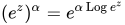
Ao longo deste artigo,
(
e
π
i
τ
)
α
{\displaystyle (e^{\pi i\tau })^{\alpha }}
e
α
π
i
τ
{\displaystyle e^{\alpha \pi i\tau }}
ramo ).[ note 1]
Existem várias funções intimamente relacionadas chamadas funções teta de Jacobi, e muitos sistemas de notação diferentes e incompatíveis para elas.
Uma função teta de Jacobi (em homenagem a Carl Gustav Jakob Jacobi ) é uma função definida para duas variáveis complexas z e τ , onde z pode ser qualquer número complexo e τ é a razão de semiperíodo , confinada ao semiplano superior , o que significa que tem uma parte imaginária positiva. É dada pela fórmula
ϑ
(
z
;
τ
)
=
∑
n
=
−
∞
∞
exp
(
π
i
n
2
τ
+
2
π
i
n
z
)
=
1
+
2
∑
n
=
1
∞
q
n
2
cos
(
2
π
n
z
)
=
∑
n
=
−
∞
∞
q
n
2
η
n
{\displaystyle {\begin{aligned}\vartheta (z;\tau )&=\sum _{n=-\infty }^{\infty }\exp \left(\pi in^{2}\tau +2\pi inz\right)\\&=1+2\sum _{n=1}^{\infty }q^{n^{2}}\cos(2\pi nz)\\&=\sum _{n=-\infty }^{\infty }q^{n^{2}}\eta ^{n}\end{aligned}}}
onde q = exp(πiτ )nomo e η = exp(2πiz )forma de Jacobi . A restrição garante que seja uma série absolutamente convergente . Em τ fixo, esta é uma série de Fourier para uma função inteira 1-periódica de z . Da mesma forma, a função teta é 1-periódica em z :
ϑ
(
z
+
1
;
τ
)
=
ϑ
(
z
;
τ
)
.
{\displaystyle \vartheta (z+1;\tau )=\vartheta (z;\tau ).}
Ao completar o quadrado , ela também é τ -quase-periódica em z , com
ϑ
(
z
+
τ
;
τ
)
=
exp
(
−
π
i
(
τ
+
2
z
)
)
ϑ
(
z
;
τ
)
.
{\displaystyle \vartheta (z+\tau ;\tau )=\exp {\bigl (}-\pi i(\tau +2z){\bigr )}\vartheta (z;\tau ).}
Assim, em geral,
ϑ
(
z
+
a
+
b
τ
;
τ
)
=
exp
(
−
π
i
b
2
τ
−
2
π
i
b
z
)
ϑ
(
z
;
τ
)
{\displaystyle \vartheta (z+a+b\tau ;\tau )=\exp \left(-\pi ib^{2}\tau -2\pi ibz\right)\vartheta (z;\tau )}
para quaisquer inteiros a e b .
Para qualquer
τ
{\displaystyle \tau }
teorema de Liouville , ela não pode ser duplamente periódica em
1
,
τ
{\displaystyle 1,\tau }
1
{\displaystyle 1}
τ
{\displaystyle \tau }
|
ϑ
(
z
+
a
+
b
τ
;
τ
)
ϑ
(
z
;
τ
)
|
=
exp
(
π
(
b
2
ℑ
(
τ
)
+
2
b
ℑ
(
z
)
)
)
{\displaystyle \left|{\frac {\vartheta (z+a+b\tau ;\tau )}{\vartheta (z;\tau )}}\right|=\exp \left(\pi (b^{2}\Im (\tau )+2b\Im (z))\right)}
ℑ
(
τ
)
>
0
{\displaystyle \Im (\tau )>0}
ϑ
(
z
,
τ
)
{\displaystyle \vartheta (z,\tau )}
Ela é de fato a função inteira mais geral com 2 quase-períodos, no seguinte sentido:[ 3]
Teorema: Se
f
:
C
→
C
{\displaystyle f:\mathbb {C} \to \mathbb {C} }
{
f
(
z
+
1
)
=
f
(
z
)
f
(
z
+
τ
)
=
e
a
z
+
2
π
i
b
f
(
z
)
{\displaystyle {\begin{cases}f(z+1)=f(z)\\f(z+\tau )=e^{az+2\pi ib}f(z)\end{cases}}}
a
,
b
∈
C
{\displaystyle a,b\in \mathbb {C} }
Se
a
=
0
{\displaystyle a=0}
b
=
τ
{\displaystyle b=\tau }
f
(
z
)
=
e
2
π
i
z
{\displaystyle f(z)=e^{2\pi iz}}
a
=
−
2
π
i
{\displaystyle a=-2\pi i}
f
(
z
)
=
C
ϑ
(
z
+
1
2
τ
+
b
,
τ
)
{\displaystyle f(z)=C\vartheta (z+{\frac {1}{2}}\tau +b,\tau )}
C
∈
C
{\displaystyle C\in \mathbb {C} }
Função teta θ 1 q = e iπτ q muda com τ Função teta θ 1 q = e iπτ q muda com τ A função teta de Jacobi definida acima é por vezes considerada juntamente com três funções teta auxiliares, caso em que é escrita com um subscrito duplo 0:
ϑ
00
(
z
;
τ
)
=
ϑ
(
z
;
τ
)
{\displaystyle \vartheta _{00}(z;\tau )=\vartheta (z;\tau )}
As funções auxiliares (ou de semiperíodo) são definidas por
ϑ
01
(
z
;
τ
)
=
ϑ
(
z
+
1
2
;
τ
)
ϑ
10
(
z
;
τ
)
=
exp
(
1
4
π
i
τ
+
π
i
z
)
ϑ
(
z
+
1
2
τ
;
τ
)
ϑ
11
(
z
;
τ
)
=
exp
(
1
4
π
i
τ
+
π
i
(
z
+
1
2
)
)
ϑ
(
z
+
1
2
τ
+
1
2
;
τ
)
.
{\displaystyle {\begin{aligned}\vartheta _{01}(z;\tau )&=\vartheta \left(z+{\tfrac {1}{2}};\tau \right)\\[3pt]\vartheta _{10}(z;\tau )&=\exp \left({\tfrac {1}{4}}\pi i\tau +\pi iz\right)\vartheta \left(z+{\tfrac {1}{2}}\tau ;\tau \right)\\[3pt]\vartheta _{11}(z;\tau )&=\exp \left({\tfrac {1}{4}}\pi i\tau +\pi i\left(z+{\tfrac {1}{2}}\right)\right)\vartheta \left(z+{\tfrac {1}{2}}\tau +{\tfrac {1}{2}};\tau \right).\end{aligned}}}
Esta notação segue Riemann e Mumford ; a formulação original de Jacobi foi em termos do nomo q = e iπτ τ . Na notação de Jacobi as funções θ são escritas:
Teta de Jacobi 1
θ
1
(
z
;
q
)
=
θ
1
(
π
z
,
q
)
=
−
ϑ
11
(
z
;
τ
)
{\displaystyle \theta _{1}(z;q)=\theta _{1}(\pi z,q)=-\vartheta _{11}(z;\tau )}
Teta de Jacobi 2
θ
2
(
z
;
q
)
=
θ
2
(
π
z
,
q
)
=
ϑ
10
(
z
;
τ
)
{\displaystyle \theta _{2}(z;q)=\theta _{2}(\pi z,q)=\vartheta _{10}(z;\tau )}
Teta de Jacobi 3
θ
3
(
z
;
q
)
=
θ
3
(
π
z
,
q
)
=
ϑ
00
(
z
;
τ
)
{\displaystyle \theta _{3}(z;q)=\theta _{3}(\pi z,q)=\vartheta _{00}(z;\tau )}
Teta de Jacobi 4
θ
4
(
z
;
q
)
=
θ
4
(
π
z
,
q
)
=
ϑ
01
(
z
;
τ
)
{\displaystyle \theta _{4}(z;q)=\theta _{4}(\pi z,q)=\vartheta _{01}(z;\tau )}
As definições acima das funções teta de Jacobi não são de forma alguma únicas. Veja Funções teta de Jacobi (variações notacionais) para uma discussão mais aprofundada.
Se definirmos z = 0τ , definidas no semiplano superior. Estas funções são chamadas de funções Theta Nullwert , com base no termo alemão para valor zero devido à anulação da entrada à esquerda na expressão da função teta. Alternativamente, obtemos quatro funções apenas de q , definidas no disco unitário
|
q
|
<
1
{\displaystyle |q|<1}
constantes teta :[ note 2]
ϑ
11
(
0
;
τ
)
=
−
θ
1
(
q
)
=
−
∑
n
=
−
∞
∞
(
−
1
)
n
−
1
/
2
q
(
n
+
1
/
2
)
2
ϑ
10
(
0
;
τ
)
=
θ
2
(
q
)
=
∑
n
=
−
∞
∞
q
(
n
+
1
/
2
)
2
ϑ
00
(
0
;
τ
)
=
θ
3
(
q
)
=
∑
n
=
−
∞
∞
q
n
2
ϑ
01
(
0
;
τ
)
=
θ
4
(
q
)
=
∑
n
=
−
∞
∞
(
−
1
)
n
q
n
2
{\displaystyle {\begin{aligned}\vartheta _{11}(0;\tau )&=-\theta _{1}(q)=-\sum _{n=-\infty }^{\infty }(-1)^{n-1/2}q^{(n+1/2)^{2}}\\\vartheta _{10}(0;\tau )&=\theta _{2}(q)=\sum _{n=-\infty }^{\infty }q^{(n+1/2)^{2}}\\\vartheta _{00}(0;\tau )&=\theta _{3}(q)=\sum _{n=-\infty }^{\infty }q^{n^{2}}\\\vartheta _{01}(0;\tau )&=\theta _{4}(q)=\sum _{n=-\infty }^{\infty }(-1)^{n}q^{n^{2}}\end{aligned}}}
com o nomo q = e iπτ
θ
1
(
q
)
=
0
{\displaystyle \theta _{1}(q)=0}
formas modulares e para parametrizar certas curvas; em particular, a identidade de Jacobi é
θ
2
(
q
)
4
+
θ
4
(
q
)
4
=
θ
3
(
q
)
4
{\displaystyle \theta _{2}(q)^{4}+\theta _{4}(q)^{4}=\theta _{3}(q)^{4}}
ou equivalentemente,
ϑ
01
(
0
;
τ
)
4
+
ϑ
10
(
0
;
τ
)
4
=
ϑ
00
(
0
;
τ
)
4
{\displaystyle \vartheta _{01}(0;\tau )^{4}+\vartheta _{10}(0;\tau )^{4}=\vartheta _{00}(0;\tau )^{4}}
que é a curva de Fermat de grau quatro.
Identidades de Jacobi
As identidades de Jacobi descrevem como as funções teta se transformam sob o grupo modular , que é gerado por τ ↦ τ + 1τ ↦ − 1 / τ τ no expoente tem o mesmo efeito que adicionar 1 / 2 z (n ≡ n 2 mod 2
α
=
(
−
i
τ
)
1
2
exp
(
π
τ
i
z
2
)
.
{\displaystyle \alpha =(-i\tau )^{\frac {1}{2}}\exp \left({\frac {\pi }{\tau }}iz^{2}\right).}
Então
ϑ
00
(
z
τ
;
−
1
τ
)
=
α
ϑ
00
(
z
;
τ
)
ϑ
01
(
z
τ
;
−
1
τ
)
=
α
ϑ
10
(
z
;
τ
)
ϑ
10
(
z
τ
;
−
1
τ
)
=
α
ϑ
01
(
z
;
τ
)
ϑ
11
(
z
τ
;
−
1
τ
)
=
−
i
α
ϑ
11
(
z
;
τ
)
.
{\displaystyle {\begin{aligned}\vartheta _{00}\!\left({\frac {z}{\tau }};{\frac {-1}{\tau }}\right)&=\alpha \,\vartheta _{00}(z;\tau )\quad &\vartheta _{01}\!\left({\frac {z}{\tau }};{\frac {-1}{\tau }}\right)&=\alpha \,\vartheta _{10}(z;\tau )\\[3pt]\vartheta _{10}\!\left({\frac {z}{\tau }};{\frac {-1}{\tau }}\right)&=\alpha \,\vartheta _{01}(z;\tau )\quad &\vartheta _{11}\!\left({\frac {z}{\tau }};{\frac {-1}{\tau }}\right)&=-i\alpha \,\vartheta _{11}(z;\tau ).\end{aligned}}}
Em vez de expressar as funções Teta em termos de z e τ , podemos expressá-las em termos dos argumentos w e o nomo q , onde w = e πiz q = e πiτ
ϑ
00
(
w
,
q
)
=
∑
n
=
−
∞
∞
(
w
2
)
n
q
n
2
ϑ
01
(
w
,
q
)
=
∑
n
=
−
∞
∞
(
−
1
)
n
(
w
2
)
n
q
n
2
ϑ
10
(
w
,
q
)
=
∑
n
=
−
∞
∞
(
w
2
)
n
+
1
2
q
(
n
+
1
2
)
2
ϑ
11
(
w
,
q
)
=
i
∑
n
=
−
∞
∞
(
−
1
)
n
(
w
2
)
n
+
1
2
q
(
n
+
1
2
)
2
.
{\displaystyle {\begin{aligned}\vartheta _{00}(w,q)&=\sum _{n=-\infty }^{\infty }\left(w^{2}\right)^{n}q^{n^{2}}\quad &\vartheta _{01}(w,q)&=\sum _{n=-\infty }^{\infty }(-1)^{n}\left(w^{2}\right)^{n}q^{n^{2}}\\[3pt]\vartheta _{10}(w,q)&=\sum _{n=-\infty }^{\infty }\left(w^{2}\right)^{n+{\frac {1}{2}}}q^{\left(n+{\frac {1}{2}}\right)^{2}}\quad &\vartheta _{11}(w,q)&=i\sum _{n=-\infty }^{\infty }(-1)^{n}\left(w^{2}\right)^{n+{\frac {1}{2}}}q^{\left(n+{\frac {1}{2}}\right)^{2}}.\end{aligned}}}
Vemos que as funções teta também podem ser definidas em termos de w e q , sem uma referência direta à função exponencial. Essas fórmulas podem, portanto, ser usadas para definir as funções Teta sobre outros corpos onde a função exponencial pode não ser definida em toda parte, como corpos de números p -ádicos .
O produto triplo de Jacobi (um caso especial das identidades de Macdonald ) nos diz que para os números complexos w e q com | q | < 1w ≠ 0
∏
m
=
1
∞
(
1
−
q
2
m
)
(
1
+
w
2
q
2
m
−
1
)
(
1
+
w
−
2
q
2
m
−
1
)
=
∑
n
=
−
∞
∞
w
2
n
q
n
2
.
{\displaystyle \prod _{m=1}^{\infty }\left(1-q^{2m}\right)\left(1+w^{2}q^{2m-1}\right)\left(1+w^{-2}q^{2m-1}\right)=\sum _{n=-\infty }^{\infty }w^{2n}q^{n^{2}}.}
Pode ser provado por meios elementares, como por exemplo no livro An Introduction to the Theory of Numbers
Se expressarmos a função teta em termos do nomo q = e πiτ q = e 2πiτ w = e πiz
ϑ
(
z
;
τ
)
=
∑
n
=
−
∞
∞
exp
(
π
i
τ
n
2
)
exp
(
2
π
i
z
n
)
=
∑
n
=
−
∞
∞
w
2
n
q
n
2
.
{\displaystyle \vartheta (z;\tau )=\sum _{n=-\infty }^{\infty }\exp(\pi i\tau n^{2})\exp(2\pi izn)=\sum _{n=-\infty }^{\infty }w^{2n}q^{n^{2}}.}
Nós, portanto, obtemos uma fórmula de produto para a função teta na forma
ϑ
(
z
;
τ
)
=
∏
m
=
1
∞
(
1
−
exp
(
2
m
π
i
τ
)
)
(
1
+
exp
(
(
2
m
−
1
)
π
i
τ
+
2
π
i
z
)
)
(
1
+
exp
(
(
2
m
−
1
)
π
i
τ
−
2
π
i
z
)
)
.
{\displaystyle \vartheta (z;\tau )=\prod _{m=1}^{\infty }{\big (}1-\exp(2m\pi i\tau ){\big )}{\Big (}1+\exp {\big (}(2m-1)\pi i\tau +2\pi iz{\big )}{\Big )}{\Big (}1+\exp {\big (}(2m-1)\pi i\tau -2\pi iz{\big )}{\Big )}.}
Em termos de w e q :
ϑ
(
z
;
τ
)
=
∏
m
=
1
∞
(
1
−
q
2
m
)
(
1
+
q
2
m
−
1
w
2
)
(
1
+
q
2
m
−
1
w
2
)
=
(
q
2
;
q
2
)
∞
(
−
w
2
q
;
q
2
)
∞
(
−
q
w
2
;
q
2
)
∞
=
(
q
2
;
q
2
)
∞
θ
(
−
w
2
q
;
q
2
)
{\displaystyle {\begin{aligned}\vartheta (z;\tau )&=\prod _{m=1}^{\infty }\left(1-q^{2m}\right)\left(1+q^{2m-1}w^{2}\right)\left(1+{\frac {q^{2m-1}}{w^{2}}}\right)\\&=\left(q^{2};q^{2}\right)_{\infty }\,\left(-w^{2}q;q^{2}\right)_{\infty }\,\left(-{\frac {q}{w^{2}}};q^{2}\right)_{\infty }\\&=\left(q^{2};q^{2}\right)_{\infty }\,\theta \left(-w^{2}q;q^{2}\right)\end{aligned}}}
onde ( ; )∞ é o símbolo q -Pochhammer e θ ( ; )função q-teta . Expandindo os termos, o produto triplo de Jacobi também pode ser escrito como
∏
m
=
1
∞
(
1
−
q
2
m
)
(
1
+
(
w
2
+
w
−
2
)
q
2
m
−
1
+
q
4
m
−
2
)
,
{\displaystyle \prod _{m=1}^{\infty }\left(1-q^{2m}\right){\Big (}1+\left(w^{2}+w^{-2}\right)q^{2m-1}+q^{4m-2}{\Big )},}
que também podemos escrever como
ϑ
(
z
∣
q
)
=
∏
m
=
1
∞
(
1
−
q
2
m
)
(
1
+
2
cos
(
2
π
z
)
q
2
m
−
1
+
q
4
m
−
2
)
.
{\displaystyle \vartheta (z\mid q)=\prod _{m=1}^{\infty }\left(1-q^{2m}\right)\left(1+2\cos(2\pi z)q^{2m-1}+q^{4m-2}\right).}
Esta forma é válida em geral, mas é claramente de particular interesse quando z é real. Fórmulas de produtos semelhantes para as funções teta auxiliares são
ϑ
01
(
z
∣
q
)
=
∏
m
=
1
∞
(
1
−
q
2
m
)
(
1
−
2
cos
(
2
π
z
)
q
2
m
−
1
+
q
4
m
−
2
)
,
ϑ
10
(
z
∣
q
)
=
2
q
1
4
cos
(
π
z
)
∏
m
=
1
∞
(
1
−
q
2
m
)
(
1
+
2
cos
(
2
π
z
)
q
2
m
+
q
4
m
)
,
ϑ
11
(
z
∣
q
)
=
−
2
q
1
4
sin
(
π
z
)
∏
m
=
1
∞
(
1
−
q
2
m
)
(
1
−
2
cos
(
2
π
z
)
q
2
m
+
q
4
m
)
.
{\displaystyle {\begin{aligned}\vartheta _{01}(z\mid q)&=\prod _{m=1}^{\infty }\left(1-q^{2m}\right)\left(1-2\cos(2\pi z)q^{2m-1}+q^{4m-2}\right),\\[3pt]\vartheta _{10}(z\mid q)&=2q^{\frac {1}{4}}\cos(\pi z)\prod _{m=1}^{\infty }\left(1-q^{2m}\right)\left(1+2\cos(2\pi z)q^{2m}+q^{4m}\right),\\[3pt]\vartheta _{11}(z\mid q)&=-2q^{\frac {1}{4}}\sin(\pi z)\prod _{m=1}^{\infty }\left(1-q^{2m}\right)\left(1-2\cos(2\pi z)q^{2m}+q^{4m}\right).\end{aligned}}}
Em particular,
lim
q
→
0
ϑ
10
(
z
∣
q
)
2
q
1
4
=
cos
(
π
z
)
,
lim
q
→
0
−
ϑ
11
(
z
∣
q
)
2
q
1
4
=
sin
(
π
z
)
{\displaystyle \lim _{q\to 0}{\frac {\vartheta _{10}(z\mid q)}{2q^{\frac {1}{4}}}}=\cos(\pi z),\quad \lim _{q\to 0}{\frac {-\vartheta _{11}(z\mid q)}{2q^{\frac {1}{4}}}}=\sin(\pi z)}
sin
,
cos
{\displaystyle \sin ,\cos }
As funções teta de Jacobi têm as seguintes representações integrais:
ϑ
00
(
z
;
τ
)
=
−
i
∫
i
−
∞
i
+
∞
e
i
π
τ
u
2
cos
(
2
π
u
z
+
π
u
)
sin
(
π
u
)
d
u
;
ϑ
01
(
z
;
τ
)
=
−
i
∫
i
−
∞
i
+
∞
e
i
π
τ
u
2
cos
(
2
π
u
z
)
sin
(
π
u
)
d
u
;
ϑ
10
(
z
;
τ
)
=
−
i
e
i
π
z
+
1
4
i
π
τ
∫
i
−
∞
i
+
∞
e
i
π
τ
u
2
cos
(
2
π
u
z
+
π
u
+
π
τ
u
)
sin
(
π
u
)
d
u
;
ϑ
11
(
z
;
τ
)
=
e
i
π
z
+
1
4
i
π
τ
∫
i
−
∞
i
+
∞
e
i
π
τ
u
2
cos
(
2
π
u
z
+
π
τ
u
)
sin
(
π
u
)
d
u
.
{\displaystyle {\begin{aligned}\vartheta _{00}(z;\tau )&=-i\int _{i-\infty }^{i+\infty }e^{i\pi \tau u^{2}}{\frac {\cos(2\pi uz+\pi u)}{\sin(\pi u)}}\mathrm {d} u;\\[6pt]\vartheta _{01}(z;\tau )&=-i\int _{i-\infty }^{i+\infty }e^{i\pi \tau u^{2}}{\frac {\cos(2\pi uz)}{\sin(\pi u)}}\mathrm {d} u;\\[6pt]\vartheta _{10}(z;\tau )&=-ie^{i\pi z+{\frac {1}{4}}i\pi \tau }\int _{i-\infty }^{i+\infty }e^{i\pi \tau u^{2}}{\frac {\cos(2\pi uz+\pi u+\pi \tau u)}{\sin(\pi u)}}\mathrm {d} u;\\[6pt]\vartheta _{11}(z;\tau )&=e^{i\pi z+{\frac {1}{4}}i\pi \tau }\int _{i-\infty }^{i+\infty }e^{i\pi \tau u^{2}}{\frac {\cos(2\pi uz+\pi \tau u)}{\sin(\pi u)}}\mathrm {d} u.\end{aligned}}}
A função Theta Nullwert
θ
3
(
q
)
{\displaystyle \theta _{3}(q)}
θ
3
(
q
)
=
1
+
4
q
ln
(
1
/
q
)
π
∫
0
∞
exp
[
−
ln
(
1
/
q
)
x
2
]
{
1
−
q
2
cos
[
2
ln
(
1
/
q
)
x
]
}
1
−
2
q
2
cos
[
2
ln
(
1
/
q
)
x
]
+
q
4
d
x
{\displaystyle \theta _{3}(q)=1+{\frac {4q{\sqrt {\ln(1/q)}}}{\sqrt {\pi }}}\int _{0}^{\infty }{\frac {\exp[-\ln(1/q)\,x^{2}]\{1-q^{2}\cos[2\ln(1/q)\,x]\}}{1-2q^{2}\cos[2\ln(1/q)\,x]+q^{4}}}\,\mathrm {d} x}
Esta fórmula foi discutida no ensaio Square series generating function transformations pelo matemático Maxie Schmidt da Geórgia, em Atlanta.
Com base nesta fórmula, os seguintes três exemplos eminentes são dados:
[
2
π
K
(
1
2
2
)
]
1
/
2
=
θ
3
[
exp
(
−
π
)
]
=
1
+
4
exp
(
−
π
)
∫
0
∞
exp
(
−
π
x
2
)
[
1
−
exp
(
−
2
π
)
cos
(
2
π
x
)
]
1
−
2
exp
(
−
2
π
)
cos
(
2
π
x
)
+
exp
(
−
4
π
)
d
x
{\displaystyle {\biggl [}{\frac {2}{\pi }}K{\bigl (}{\frac {1}{2}}{\sqrt {2}}{\bigr )}{\biggr ]}^{1/2}=\theta _{3}{\bigl [}\exp(-\pi ){\bigr ]}=1+4\exp(-\pi )\int _{0}^{\infty }{\frac {\exp(-\pi x^{2})[1-\exp(-2\pi )\cos(2\pi x)]}{1-2\exp(-2\pi )\cos(2\pi x)+\exp(-4\pi )}}\,\mathrm {d} x}
[
2
π
K
(
2
−
1
)
]
1
/
2
=
θ
3
[
exp
(
−
2
π
)
]
=
1
+
4
2
4
exp
(
−
2
π
)
∫
0
∞
exp
(
−
2
π
x
2
)
[
1
−
exp
(
−
2
2
π
)
cos
(
2
2
π
x
)
]
1
−
2
exp
(
−
2
2
π
)
cos
(
2
2
π
x
)
+
exp
(
−
4
2
π
)
d
x
{\displaystyle {\biggl [}{\frac {2}{\pi }}K({\sqrt {2}}-1){\biggr ]}^{1/2}=\theta _{3}{\bigl [}\exp(-{\sqrt {2}}\,\pi ){\bigr ]}=1+4\,{\sqrt[{4}]{2}}\exp(-{\sqrt {2}}\,\pi )\int _{0}^{\infty }{\frac {\exp(-{\sqrt {2}}\,\pi x^{2})[1-\exp(-2{\sqrt {2}}\,\pi )\cos(2{\sqrt {2}}\,\pi x)]}{1-2\exp(-2{\sqrt {2}}\,\pi )\cos(2{\sqrt {2}}\,\pi x)+\exp(-4{\sqrt {2}}\,\pi )}}\,\mathrm {d} x}
{
2
π
K
[
sin
(
π
12
)
]
}
1
/
2
=
θ
3
[
exp
(
−
3
π
)
]
=
1
+
4
3
4
exp
(
−
3
π
)
∫
0
∞
exp
(
−
3
π
x
2
)
[
1
−
exp
(
−
2
3
π
)
cos
(
2
3
π
x
)
]
1
−
2
exp
(
−
2
3
π
)
cos
(
2
3
π
x
)
+
exp
(
−
4
3
π
)
d
x
{\displaystyle {\biggl \{}{\frac {2}{\pi }}K{\bigl [}\sin {\bigl (}{\frac {\pi }{12}}{\bigr )}{\bigr ]}{\biggr \}}^{1/2}=\theta _{3}{\bigl [}\exp(-{\sqrt {3}}\,\pi ){\bigr ]}=1+4\,{\sqrt[{4}]{3}}\exp(-{\sqrt {3}}\,\pi )\int _{0}^{\infty }{\frac {\exp(-{\sqrt {3}}\,\pi x^{2})[1-\exp(-2{\sqrt {3}}\,\pi )\cos(2{\sqrt {3}}\,\pi x)]}{1-2\exp(-2{\sqrt {3}}\,\pi )\cos(2{\sqrt {3}}\,\pi x)+\exp(-4{\sqrt {3}}\,\pi )}}\,\mathrm {d} x}
Além disso, os exemplos da função teta
θ
3
(
1
2
)
{\displaystyle \theta _{3}({\tfrac {1}{2}})}
θ
3
(
1
3
)
{\displaystyle \theta _{3}({\tfrac {1}{3}})}
θ
3
(
1
2
)
=
1
+
2
∑
n
=
1
∞
1
2
n
2
=
1
+
2
π
−
1
/
2
ln
(
2
)
∫
0
∞
exp
[
−
ln
(
2
)
x
2
]
{
16
−
4
cos
[
2
ln
(
2
)
x
]
}
17
−
8
cos
[
2
ln
(
2
)
x
]
d
x
{\displaystyle \theta _{3}\left({\frac {1}{2}}\right)=1+2\sum _{n=1}^{\infty }{\frac {1}{2^{n^{2}}}}=1+2\pi ^{-1/2}{\sqrt {\ln(2)}}\int _{0}^{\infty }{\frac {\exp[-\ln(2)\,x^{2}]\{16-4\cos[2\ln(2)\,x]\}}{17-8\cos[2\ln(2)\,x]}}\,\mathrm {d} x}
θ
3
(
1
2
)
=
2.128936827211877158669
…
{\displaystyle \theta _{3}\left({\frac {1}{2}}\right)=2.128936827211877158669\ldots }
θ
3
(
1
3
)
=
1
+
2
∑
n
=
1
∞
1
3
n
2
=
1
+
4
3
π
−
1
/
2
ln
(
3
)
∫
0
∞
exp
[
−
ln
(
3
)
x
2
]
{
81
−
9
cos
[
2
ln
(
3
)
x
]
}
82
−
18
cos
[
2
ln
(
3
)
x
]
d
x
{\displaystyle \theta _{3}\left({\frac {1}{3}}\right)=1+2\sum _{n=1}^{\infty }{\frac {1}{3^{n^{2}}}}=1+{\frac {4}{3}}\pi ^{-1/2}{\sqrt {\ln(3)}}\int _{0}^{\infty }{\frac {\exp[-\ln(3)\,x^{2}]\{81-9\cos[2\ln(3)\,x]\}}{82-18\cos[2\ln(3)\,x]}}\,\mathrm {d} x}
θ
3
(
1
3
)
=
1.691459681681715341348
…
{\displaystyle \theta _{3}\left({\frac {1}{3}}\right)=1.691459681681715341348\ldots }
O devido crédito pela maioria desses resultados pertence a Ramanujan. Veja Caderno perdido de Ramanujan e uma referência relevante em Função de Euler . Os resultados de Ramanujan citados em Função de Euler somados a algumas operações elementares geram os resultados abaixo, de modo que eles estão no caderno perdido de Ramanujan ou decorrem imediatamente dele. Veja também Yi (2004).[ 4]
φ
(
q
)
=
ϑ
00
(
0
;
τ
)
=
θ
3
(
0
;
q
)
=
∑
n
=
−
∞
∞
q
n
2
{\displaystyle \quad \varphi (q)=\vartheta _{00}(0;\tau )=\theta _{3}(0;q)=\sum _{n=-\infty }^{\infty }q^{n^{2}}}
com o nomo
q
=
e
π
i
τ
,
{\displaystyle q=e^{\pi i\tau },}
τ
=
n
−
1
,
{\displaystyle \tau =n{\sqrt {-1}},}
função eta de Dedekind
η
(
τ
)
.
{\displaystyle \eta (\tau ).}
n
=
1
,
2
,
3
,
…
{\displaystyle n=1,2,3,\dots }
φ
(
e
−
π
)
=
π
4
Γ
(
3
4
)
=
2
η
(
−
1
)
φ
(
e
−
2
π
)
=
π
4
Γ
(
3
4
)
2
+
2
2
φ
(
e
−
3
π
)
=
π
4
Γ
(
3
4
)
1
+
3
108
8
φ
(
e
−
4
π
)
=
π
4
Γ
(
3
4
)
2
+
8
4
4
φ
(
e
−
5
π
)
=
π
4
Γ
(
3
4
)
2
+
5
5
φ
(
e
−
6
π
)
=
π
4
Γ
(
3
4
)
1
4
+
3
4
+
4
4
+
9
4
12
3
8
φ
(
e
−
7
π
)
=
π
4
Γ
(
3
4
)
13
+
7
+
7
+
3
7
14
3
8
⋅
7
16
φ
(
e
−
8
π
)
=
π
4
Γ
(
3
4
)
2
+
2
+
128
8
4
φ
(
e
−
9
π
)
=
π
4
Γ
(
3
4
)
1
+
2
+
2
3
3
3
φ
(
e
−
10
π
)
=
π
4
Γ
(
3
4
)
64
4
+
80
4
+
81
4
+
100
4
200
4
φ
(
e
−
11
π
)
=
π
4
Γ
(
3
4
)
11
+
11
+
(
5
+
3
3
+
11
+
33
)
−
44
+
33
3
3
+
(
−
5
+
3
3
−
11
+
33
)
44
+
33
3
3
52180524
8
φ
(
e
−
12
π
)
=
π
4
Γ
(
3
4
)
1
4
+
2
4
+
3
4
+
4
4
+
9
4
+
18
4
+
24
4
2
108
8
φ
(
e
−
13
π
)
=
π
4
Γ
(
3
4
)
13
+
8
13
+
(
11
−
6
3
+
13
)
143
+
78
3
3
+
(
11
+
6
3
+
13
)
143
−
78
3
3
19773
4
φ
(
e
−
14
π
)
=
π
4
Γ
(
3
4
)
13
+
7
+
7
+
3
7
+
10
+
2
7
+
28
8
4
+
7
28
7
16
φ
(
e
−
15
π
)
=
π
4
Γ
(
3
4
)
7
+
3
3
+
5
+
15
+
60
4
+
1500
4
12
3
8
⋅
5
2
φ
(
e
−
16
π
)
=
φ
(
e
−
4
π
)
+
π
4
Γ
(
3
4
)
1
+
2
4
128
16
φ
(
e
−
17
π
)
=
π
4
Γ
(
3
4
)
2
(
1
+
17
4
)
+
17
8
5
+
17
17
+
17
17
2
φ
(
e
−
20
π
)
=
φ
(
e
−
5
π
)
+
π
4
Γ
(
3
4
)
3
+
2
5
4
5
2
6
φ
(
e
−
36
π
)
=
3
φ
(
e
−
9
π
)
+
2
φ
(
e
−
4
π
)
−
φ
(
e
−
π
)
+
π
4
Γ
(
3
4
)
2
4
+
18
4
+
216
4
3
{\displaystyle {\begin{aligned}\varphi \left(e^{-\pi }\right)&={\frac {\sqrt[{4}]{\pi }}{\Gamma \left({\frac {3}{4}}\right)}}={\sqrt {2}}\,\eta \left({\sqrt {-1}}\right)\\\varphi \left(e^{-2\pi }\right)&={\frac {\sqrt[{4}]{\pi }}{\Gamma \left({\frac {3}{4}}\right)}}{\frac {\sqrt {2+{\sqrt {2}}}}{2}}\\\varphi \left(e^{-3\pi }\right)&={\frac {\sqrt[{4}]{\pi }}{\Gamma \left({\frac {3}{4}}\right)}}{\frac {\sqrt {1+{\sqrt {3}}}}{\sqrt[{8}]{108}}}\\\varphi \left(e^{-4\pi }\right)&={\frac {\sqrt[{4}]{\pi }}{\Gamma \left({\frac {3}{4}}\right)}}{\frac {2+{\sqrt[{4}]{8}}}{4}}\\\varphi \left(e^{-5\pi }\right)&={\frac {\sqrt[{4}]{\pi }}{\Gamma \left({\frac {3}{4}}\right)}}{\sqrt {\frac {2+{\sqrt {5}}}{5}}}\\\varphi \left(e^{-6\pi }\right)&={\frac {\sqrt[{4}]{\pi }}{\Gamma \left({\frac {3}{4}}\right)}}{\frac {\sqrt {{\sqrt[{4}]{1}}+{\sqrt[{4}]{3}}+{\sqrt[{4}]{4}}+{\sqrt[{4}]{9}}}}{\sqrt[{8}]{12^{3}}}}\\\varphi \left(e^{-7\pi }\right)&={\frac {\sqrt[{4}]{\pi }}{\Gamma \left({\frac {3}{4}}\right)}}{\frac {\sqrt {{\sqrt {13+{\sqrt {7}}}}+{\sqrt {7+3{\sqrt {7}}}}}}{{\sqrt[{8}]{14^{3}}}\cdot {\sqrt[{16}]{7}}}}\\\varphi \left(e^{-8\pi }\right)&={\frac {\sqrt[{4}]{\pi }}{\Gamma \left({\frac {3}{4}}\right)}}{\frac {{\sqrt {2+{\sqrt {2}}}}+{\sqrt[{8}]{128}}}{4}}\\\varphi \left(e^{-9\pi }\right)&={\frac {\sqrt[{4}]{\pi }}{\Gamma \left({\frac {3}{4}}\right)}}{\frac {1+{\sqrt[{3}]{2+2{\sqrt {3}}}}}{3}}\\\varphi \left(e^{-10\pi }\right)&={\frac {\sqrt[{4}]{\pi }}{\Gamma \left({\frac {3}{4}}\right)}}{\frac {\sqrt {{\sqrt[{4}]{64}}+{\sqrt[{4}]{80}}+{\sqrt[{4}]{81}}+{\sqrt[{4}]{100}}}}{\sqrt[{4}]{200}}}\\\varphi \left(e^{-11\pi }\right)&={\frac {\sqrt[{4}]{\pi }}{\Gamma \left({\frac {3}{4}}\right)}}{\frac {\sqrt {11+{\sqrt {11}}+(5+3{\sqrt {3}}+{\sqrt {11}}+{\sqrt {33}}){\sqrt[{3}]{-44+33{\sqrt {3}}}}+(-5+3{\sqrt {3}}-{\sqrt {11}}+{\sqrt {33}}){\sqrt[{3}]{44+33{\sqrt {3}}}}}}{\sqrt[{8}]{52180524}}}\\\varphi \left(e^{-12\pi }\right)&={\frac {\sqrt[{4}]{\pi }}{\Gamma \left({\frac {3}{4}}\right)}}{\frac {\sqrt {{\sqrt[{4}]{1}}+{\sqrt[{4}]{2}}+{\sqrt[{4}]{3}}+{\sqrt[{4}]{4}}+{\sqrt[{4}]{9}}+{\sqrt[{4}]{18}}+{\sqrt[{4}]{24}}}}{2{\sqrt[{8}]{108}}}}\\\varphi \left(e^{-13\pi }\right)&={\frac {\sqrt[{4}]{\pi }}{\Gamma \left({\frac {3}{4}}\right)}}{\frac {\sqrt {13+8{\sqrt {13}}+(11-6{\sqrt {3}}+{\sqrt {13}}){\sqrt[{3}]{143+78{\sqrt {3}}}}+(11+6{\sqrt {3}}+{\sqrt {13}}){\sqrt[{3}]{143-78{\sqrt {3}}}}}}{\sqrt[{4}]{19773}}}\\\varphi \left(e^{-14\pi }\right)&={\frac {\sqrt[{4}]{\pi }}{\Gamma \left({\frac {3}{4}}\right)}}{\frac {\sqrt {{\sqrt {13+{\sqrt {7}}}}+{\sqrt {7+3{\sqrt {7}}}}+{\sqrt {10+2{\sqrt {7}}}}+{\sqrt[{8}]{28}}{\sqrt {4+{\sqrt {7}}}}}}{\sqrt[{16}]{28^{7}}}}\\\varphi \left(e^{-15\pi }\right)&={\frac {\sqrt[{4}]{\pi }}{\Gamma \left({\frac {3}{4}}\right)}}{\frac {\sqrt {7+3{\sqrt {3}}+{\sqrt {5}}+{\sqrt {15}}+{\sqrt[{4}]{60}}+{\sqrt[{4}]{1500}}}}{{\sqrt[{8}]{12^{3}}}\cdot {\sqrt {5}}}}\\2\varphi \left(e^{-16\pi }\right)&=\varphi \left(e^{-4\pi }\right)+{\frac {\sqrt[{4}]{\pi }}{\Gamma \left({\frac {3}{4}}\right)}}{\frac {\sqrt[{4}]{1+{\sqrt {2}}}}{\sqrt[{16}]{128}}}\\\varphi \left(e^{-17\pi }\right)&={\frac {\sqrt[{4}]{\pi }}{\Gamma \left({\frac {3}{4}}\right)}}{\frac {{\sqrt {2}}(1+{\sqrt[{4}]{17}})+{\sqrt[{8}]{17}}{\sqrt {5+{\sqrt {17}}}}}{\sqrt {17+17{\sqrt {17}}}}}\\2\varphi \left(e^{-20\pi }\right)&=\varphi \left(e^{-5\pi }\right)+{\frac {\sqrt[{4}]{\pi }}{\Gamma \left({\frac {3}{4}}\right)}}{\sqrt {\frac {3+2{\sqrt[{4}]{5}}}{5{\sqrt {2}}}}}\\6\varphi \left(e^{-36\pi }\right)&=3\varphi \left(e^{-9\pi }\right)+2\varphi \left(e^{-4\pi }\right)-\varphi \left(e^{-\pi }\right)+{\frac {\sqrt[{4}]{\pi }}{\Gamma \left({\frac {3}{4}}\right)}}{\sqrt[{3}]{{\sqrt[{4}]{2}}+{\sqrt[{4}]{18}}+{\sqrt[{4}]{216}}}}\end{aligned}}}
Se o recíproco da constante de Gelfond for elevado à potência do recíproco de um número ímpar, então os valores correspondentes de
ϑ
00
{\displaystyle \vartheta _{00}}
ϕ
{\displaystyle \phi }
seno lemniscático hiperbólico :
φ
[
exp
(
−
1
5
π
)
]
=
π
4
Γ
(
3
4
)
−
1
slh
(
1
5
2
ϖ
)
slh
(
2
5
2
ϖ
)
{\displaystyle \varphi {\bigl [}\exp(-{\tfrac {1}{5}}\pi ){\bigr ]}={\sqrt[{4}]{\pi }}\,{\Gamma \left({\tfrac {3}{4}}\right)}^{-1}\operatorname {slh} {\bigl (}{\tfrac {1}{5}}{\sqrt {2}}\,\varpi {\bigr )}\operatorname {slh} {\bigl (}{\tfrac {2}{5}}{\sqrt {2}}\,\varpi {\bigr )}}
φ
[
exp
(
−
1
7
π
)
]
=
π
4
Γ
(
3
4
)
−
1
slh
(
1
7
2
ϖ
)
slh
(
2
7
2
ϖ
)
slh
(
3
7
2
ϖ
)
{\displaystyle \varphi {\bigl [}\exp(-{\tfrac {1}{7}}\pi ){\bigr ]}={\sqrt[{4}]{\pi }}\,{\Gamma \left({\tfrac {3}{4}}\right)}^{-1}\operatorname {slh} {\bigl (}{\tfrac {1}{7}}{\sqrt {2}}\,\varpi {\bigr )}\operatorname {slh} {\bigl (}{\tfrac {2}{7}}{\sqrt {2}}\,\varpi {\bigr )}\operatorname {slh} {\bigl (}{\tfrac {3}{7}}{\sqrt {2}}\,\varpi {\bigr )}}
φ
[
exp
(
−
1
9
π
)
]
=
π
4
Γ
(
3
4
)
−
1
slh
(
1
9
2
ϖ
)
slh
(
2
9
2
ϖ
)
slh
(
3
9
2
ϖ
)
slh
(
4
9
2
ϖ
)
{\displaystyle \varphi {\bigl [}\exp(-{\tfrac {1}{9}}\pi ){\bigr ]}={\sqrt[{4}]{\pi }}\,{\Gamma \left({\tfrac {3}{4}}\right)}^{-1}\operatorname {slh} {\bigl (}{\tfrac {1}{9}}{\sqrt {2}}\,\varpi {\bigr )}\operatorname {slh} {\bigl (}{\tfrac {2}{9}}{\sqrt {2}}\,\varpi {\bigr )}\operatorname {slh} {\bigl (}{\tfrac {3}{9}}{\sqrt {2}}\,\varpi {\bigr )}\operatorname {slh} {\bigl (}{\tfrac {4}{9}}{\sqrt {2}}\,\varpi {\bigr )}}
φ
[
exp
(
−
1
11
π
)
]
=
π
4
Γ
(
3
4
)
−
1
slh
(
1
11
2
ϖ
)
slh
(
2
11
2
ϖ
)
slh
(
3
11
2
ϖ
)
slh
(
4
11
2
ϖ
)
slh
(
5
11
2
ϖ
)
{\displaystyle \varphi {\bigl [}\exp(-{\tfrac {1}{11}}\pi ){\bigr ]}={\sqrt[{4}]{\pi }}\,{\Gamma \left({\tfrac {3}{4}}\right)}^{-1}\operatorname {slh} {\bigl (}{\tfrac {1}{11}}{\sqrt {2}}\,\varpi {\bigr )}\operatorname {slh} {\bigl (}{\tfrac {2}{11}}{\sqrt {2}}\,\varpi {\bigr )}\operatorname {slh} {\bigl (}{\tfrac {3}{11}}{\sqrt {2}}\,\varpi {\bigr )}\operatorname {slh} {\bigl (}{\tfrac {4}{11}}{\sqrt {2}}\,\varpi {\bigr )}\operatorname {slh} {\bigl (}{\tfrac {5}{11}}{\sqrt {2}}\,\varpi {\bigr )}}
A letra
ϖ
{\displaystyle \varpi }
constante da lemniscata .
Note que as seguintes identidades modulares são válidas:
2
φ
(
q
4
)
=
φ
(
q
)
+
2
φ
2
(
q
2
)
−
φ
2
(
q
)
3
φ
(
q
9
)
=
φ
(
q
)
+
9
φ
4
(
q
3
)
φ
(
q
)
−
φ
3
(
q
)
3
5
φ
(
q
25
)
=
φ
(
q
5
)
cot
(
1
2
arctan
(
2
5
φ
(
q
)
φ
(
q
5
)
φ
2
(
q
)
−
φ
2
(
q
5
)
1
+
s
(
q
)
−
s
2
(
q
)
s
(
q
)
)
)
{\displaystyle {\begin{aligned}2\varphi \left(q^{4}\right)&=\varphi (q)+{\sqrt {2\varphi ^{2}\left(q^{2}\right)-\varphi ^{2}(q)}}\\3\varphi \left(q^{9}\right)&=\varphi (q)+{\sqrt[{3}]{9{\frac {\varphi ^{4}\left(q^{3}\right)}{\varphi (q)}}-\varphi ^{3}(q)}}\\{\sqrt {5}}\varphi \left(q^{25}\right)&=\varphi \left(q^{5}\right)\cot \left({\frac {1}{2}}\arctan \left({\frac {2}{\sqrt {5}}}{\frac {\varphi (q)\varphi \left(q^{5}\right)}{\varphi ^{2}(q)-\varphi ^{2}\left(q^{5}\right)}}{\frac {1+s(q)-s^{2}(q)}{s(q)}}\right)\right)\end{aligned}}}
onde
s
(
q
)
=
s
(
e
π
i
τ
)
=
−
R
(
−
e
−
π
i
/
(
5
τ
)
)
{\displaystyle s(q)=s\left(e^{\pi i\tau }\right)=-R\left(-e^{-\pi i/(5\tau )}\right)}
fração contínua de Rogers-Ramanujan :
s
(
q
)
=
tan
(
1
2
arctan
(
5
2
φ
2
(
q
5
)
φ
2
(
q
)
−
1
2
)
)
cot
2
(
1
2
arccot
(
5
2
φ
2
(
q
5
)
φ
2
(
q
)
−
1
2
)
)
5
=
e
−
π
i
/
(
25
τ
)
1
−
e
−
π
i
/
(
5
τ
)
1
+
e
−
2
π
i
/
(
5
τ
)
1
−
⋱
{\displaystyle {\begin{aligned}s(q)&={\sqrt[{5}]{\tan \left({\frac {1}{2}}\arctan \left({\frac {5}{2}}{\frac {\varphi ^{2}\left(q^{5}\right)}{\varphi ^{2}(q)}}-{\frac {1}{2}}\right)\right)\cot ^{2}\left({\frac {1}{2}}\operatorname {arccot} \left({\frac {5}{2}}{\frac {\varphi ^{2}\left(q^{5}\right)}{\varphi ^{2}(q)}}-{\frac {1}{2}}\right)\right)}}\\&={\cfrac {e^{-\pi i/(25\tau )}}{1-{\cfrac {e^{-\pi i/(5\tau )}}{1+{\cfrac {e^{-2\pi i/(5\tau )}}{1-\ddots }}}}}}\end{aligned}}}
O matemático Bruce Berndt encontrou valores adicionais[ 5]
φ
(
exp
(
−
3
π
)
)
=
π
−
1
Γ
(
4
3
)
3
/
2
2
−
2
/
3
3
13
/
8
φ
(
exp
(
−
2
3
π
)
)
=
π
−
1
Γ
(
4
3
)
3
/
2
2
−
2
/
3
3
13
/
8
cos
(
1
24
π
)
φ
(
exp
(
−
3
3
π
)
)
=
π
−
1
Γ
(
4
3
)
3
/
2
2
−
2
/
3
3
7
/
8
(
2
3
+
1
)
φ
(
exp
(
−
4
3
π
)
)
=
π
−
1
Γ
(
4
3
)
3
/
2
2
−
5
/
3
3
13
/
8
(
1
+
cos
(
1
12
π
)
)
φ
(
exp
(
−
5
3
π
)
)
=
π
−
1
Γ
(
4
3
)
3
/
2
2
−
2
/
3
3
5
/
8
sin
(
1
5
π
)
(
2
5
100
3
+
2
5
10
3
+
3
5
5
+
1
)
{\displaystyle {\begin{array}{lll}\varphi \left(\exp(-{\sqrt {3}}\,\pi )\right)&=&\pi ^{-1}{\Gamma \left({\tfrac {4}{3}}\right)}^{3/2}2^{-2/3}3^{13/8}\\\varphi \left(\exp(-2{\sqrt {3}}\,\pi )\right)&=&\pi ^{-1}{\Gamma \left({\tfrac {4}{3}}\right)}^{3/2}2^{-2/3}3^{13/8}\cos({\tfrac {1}{24}}\pi )\\\varphi \left(\exp(-3{\sqrt {3}}\,\pi )\right)&=&\pi ^{-1}{\Gamma \left({\tfrac {4}{3}}\right)}^{3/2}2^{-2/3}3^{7/8}({\sqrt[{3}]{2}}+1)\\\varphi \left(\exp(-4{\sqrt {3}}\,\pi )\right)&=&\pi ^{-1}{\Gamma \left({\tfrac {4}{3}}\right)}^{3/2}2^{-5/3}3^{13/8}{\Bigl (}1+{\sqrt {\cos({\tfrac {1}{12}}\pi )}}{\Bigr )}\\\varphi \left(\exp(-5{\sqrt {3}}\,\pi )\right)&=&\pi ^{-1}{\Gamma \left({\tfrac {4}{3}}\right)}^{3/2}2^{-2/3}3^{5/8}\sin({\tfrac {1}{5}}\pi )({\tfrac {2}{5}}{\sqrt[{3}]{100}}+{\tfrac {2}{5}}{\sqrt[{3}]{10}}+{\tfrac {3}{5}}{\sqrt {5}}+1)\end{array}}}
Para a transformação do nomo[ 6]
θ
2
(
q
2
)
=
1
2
2
[
θ
3
(
q
)
2
−
θ
4
(
q
)
2
]
{\displaystyle \theta _{2}(q^{2})={\tfrac {1}{2}}{\sqrt {2[\theta _{3}(q)^{2}-\theta _{4}(q)^{2}]}}}
θ
3
(
q
2
)
=
1
2
2
[
θ
3
(
q
)
2
+
θ
4
(
q
)
2
]
{\displaystyle \theta _{3}(q^{2})={\tfrac {1}{2}}{\sqrt {2[\theta _{3}(q)^{2}+\theta _{4}(q)^{2}]}}}
θ
4
(
q
2
)
=
θ
4
(
q
)
θ
3
(
q
)
{\displaystyle \theta _{4}(q^{2})={\sqrt {\theta _{4}(q)\theta _{3}(q)}}}
Os quadrados das três funções teta com valor nulo, com a função quadrática como função interna, também são formados no padrão das trincas pitagóricas de acordo com a identidade de Jacobi . Além disso, as seguintes transformações são válidas:
θ
3
(
q
4
)
=
1
2
θ
3
(
q
)
+
1
2
θ
4
(
q
)
{\displaystyle \theta _{3}(q^{4})={\tfrac {1}{2}}\theta _{3}(q)+{\tfrac {1}{2}}\theta _{4}(q)}
Estas fórmulas podem ser usadas para computar os valores teta do cubo do nomo:
27
θ
3
(
q
3
)
8
−
18
θ
3
(
q
3
)
4
θ
3
(
q
)
4
−
θ
3
(
q
)
8
=
8
θ
3
(
q
3
)
2
θ
3
(
q
)
2
[
2
θ
4
(
q
)
4
−
θ
3
(
q
)
4
]
{\displaystyle 27\,\theta _{3}(q^{3})^{8}-18\,\theta _{3}(q^{3})^{4}\theta _{3}(q)^{4}-\,\theta _{3}(q)^{8}=8\,\theta _{3}(q^{3})^{2}\theta _{3}(q)^{2}[2\,\theta _{4}(q)^{4}-\theta _{3}(q)^{4}]}
27
θ
4
(
q
3
)
8
−
18
θ
4
(
q
3
)
4
θ
4
(
q
)
4
−
θ
4
(
q
)
8
=
8
θ
4
(
q
3
)
2
θ
4
(
q
)
2
[
2
θ
3
(
q
)
4
−
θ
4
(
q
)
4
]
{\displaystyle 27\,\theta _{4}(q^{3})^{8}-18\,\theta _{4}(q^{3})^{4}\theta _{4}(q)^{4}-\,\theta _{4}(q)^{8}=8\,\theta _{4}(q^{3})^{2}\theta _{4}(q)^{2}[2\,\theta _{3}(q)^{4}-\theta _{4}(q)^{4}]}
E as seguintes fórmulas podem ser usadas para computar os valores teta da quinta potência do nomo:
[
θ
3
(
q
)
2
−
θ
3
(
q
5
)
2
]
[
5
θ
3
(
q
5
)
2
−
θ
3
(
q
)
2
]
5
=
256
θ
3
(
q
5
)
2
θ
3
(
q
)
2
θ
4
(
q
)
4
[
θ
3
(
q
)
4
−
θ
4
(
q
)
4
]
{\displaystyle [\theta _{3}(q)^{2}-\theta _{3}(q^{5})^{2}][5\,\theta _{3}(q^{5})^{2}-\theta _{3}(q)^{2}]^{5}=256\,\theta _{3}(q^{5})^{2}\theta _{3}(q)^{2}\theta _{4}(q)^{4}[\theta _{3}(q)^{4}-\theta _{4}(q)^{4}]}
[
θ
4
(
q
5
)
2
−
θ
4
(
q
)
2
]
[
5
θ
4
(
q
5
)
2
−
θ
4
(
q
)
2
]
5
=
256
θ
4
(
q
5
)
2
θ
4
(
q
)
2
θ
3
(
q
)
4
[
θ
3
(
q
)
4
−
θ
4
(
q
)
4
]
{\displaystyle [\theta _{4}(q^{5})^{2}-\theta _{4}(q)^{2}][5\,\theta _{4}(q^{5})^{2}-\theta _{4}(q)^{2}]^{5}=256\,\theta _{4}(q^{5})^{2}\theta _{4}(q)^{2}\theta _{3}(q)^{4}[\theta _{3}(q)^{4}-\theta _{4}(q)^{4}]}
As fórmulas para os valores da função teta *Nullwert* a partir da raiz cúbica do nomo elíptico são obtidas contrapondo as duas soluções reais das equações quárticas correspondentes:
[
θ
3
(
q
1
/
3
)
2
θ
3
(
q
)
2
−
3
θ
3
(
q
3
)
2
θ
3
(
q
)
2
]
2
=
4
−
4
[
2
θ
2
(
q
)
2
θ
4
(
q
)
2
θ
3
(
q
)
4
]
2
/
3
{\displaystyle {\biggl [}{\frac {\theta _{3}(q^{1/3})^{2}}{\theta _{3}(q)^{2}}}-{\frac {3\,\theta _{3}(q^{3})^{2}}{\theta _{3}(q)^{2}}}{\biggr ]}^{2}=4-4{\biggl [}{\frac {2\,\theta _{2}(q)^{2}\theta _{4}(q)^{2}}{\theta _{3}(q)^{4}}}{\biggr ]}^{2/3}}
[
3
θ
4
(
q
3
)
2
θ
4
(
q
)
2
−
θ
4
(
q
1
/
3
)
2
θ
4
(
q
)
2
]
2
=
4
+
4
[
2
θ
2
(
q
)
2
θ
3
(
q
)
2
θ
4
(
q
)
4
]
2
/
3
{\displaystyle {\biggl [}{\frac {3\,\theta _{4}(q^{3})^{2}}{\theta _{4}(q)^{2}}}-{\frac {\theta _{4}(q^{1/3})^{2}}{\theta _{4}(q)^{2}}}{\biggr ]}^{2}=4+4{\biggl [}{\frac {2\,\theta _{2}(q)^{2}\theta _{3}(q)^{2}}{\theta _{4}(q)^{4}}}{\biggr ]}^{2/3}}
Em combinação com o módulo elíptico, as seguintes fórmulas podem ser exibidas:
Estas são as fórmulas para o quadrado do nomo elíptico:
θ
4
[
q
(
k
)
]
=
θ
4
[
q
(
k
)
2
]
1
−
k
2
8
{\displaystyle \theta _{4}[q(k)]=\theta _{4}[q(k)^{2}]{\sqrt[{8}]{1-k^{2}}}}
θ
4
[
q
(
k
)
2
]
=
θ
3
[
q
(
k
)
]
1
−
k
2
8
{\displaystyle \theta _{4}[q(k)^{2}]=\theta _{3}[q(k)]{\sqrt[{8}]{1-k^{2}}}}
θ
3
[
q
(
k
)
2
]
=
θ
3
[
q
(
k
)
]
cos
[
1
2
arcsin
(
k
)
]
{\displaystyle \theta _{3}[q(k)^{2}]=\theta _{3}[q(k)]\cos[{\tfrac {1}{2}}\arcsin(k)]}
E esta é uma fórmula eficiente para o cubo do nomo:
θ
4
⟨
q
{
tan
[
1
2
arctan
(
t
3
)
]
}
3
⟩
=
θ
4
⟨
q
{
tan
[
1
2
arctan
(
t
3
)
]
}
⟩
3
−
1
/
2
(
2
t
4
−
t
2
+
1
−
t
2
+
2
+
t
2
+
1
)
1
/
2
{\displaystyle \theta _{4}{\biggl \langle }q{\bigl \{}\tan {\bigl [}{\tfrac {1}{2}}\arctan(t^{3}){\bigr ]}{\bigr \}}^{3}{\biggr \rangle }=\theta _{4}{\biggl \langle }q{\bigl \{}\tan {\bigl [}{\tfrac {1}{2}}\arctan(t^{3}){\bigr ]}{\bigr \}}{\biggr \rangle }\,3^{-1/2}{\bigl (}{\sqrt {2{\sqrt {t^{4}-t^{2}+1}}-t^{2}+2}}+{\sqrt {t^{2}+1}}\,{\bigr )}^{1/2}}
Para todos os valores reais
t
∈
R
{\displaystyle t\in \mathbb {R} }
E para esta fórmula, dois exemplos serão dados:
Primeiro exemplo de cálculo com o valor
t
=
1
{\displaystyle t=1}
θ
4
⟨
q
{
tan
[
1
2
arctan
(
1
)
]
}
3
⟩
=
θ
4
⟨
q
{
tan
[
1
2
arctan
(
1
)
]
}
⟩
3
−
1
/
2
(
3
+
2
)
1
/
2
{\displaystyle \theta _{4}{\biggl \langle }q{\bigl \{}\tan {\bigl [}{\tfrac {1}{2}}\arctan(1){\bigr ]}{\bigr \}}^{3}{\biggr \rangle }=\theta _{4}{\biggl \langle }q{\bigl \{}\tan {\bigl [}{\tfrac {1}{2}}\arctan(1){\bigr ]}{\bigr \}}{\biggr \rangle }\,3^{-1/2}{\bigl (}{\sqrt {3}}+{\sqrt {2}}\,{\bigr )}^{1/2}}
θ
4
[
exp
(
−
3
2
π
)
]
=
θ
4
[
exp
(
−
2
π
)
]
3
−
1
/
2
(
3
+
2
)
1
/
2
{\displaystyle \theta _{4}{\bigl [}\exp(-3{\sqrt {2}}\,\pi ){\bigr ]}=\theta _{4}{\bigl [}\exp(-{\sqrt {2}}\,\pi ){\bigr ]}\,3^{-1/2}{\bigl (}{\sqrt {3}}+{\sqrt {2}}\,{\bigr )}^{1/2}}
Segundo exemplo de cálculo com o valor
t
=
Φ
−
2
{\displaystyle t=\Phi ^{-2}}
θ
4
⟨
q
{
tan
[
1
2
arctan
(
Φ
−
6
)
]
}
3
⟩
=
θ
4
⟨
q
{
tan
[
1
2
arctan
(
Φ
−
6
)
]
}
⟩
3
−
1
/
2
(
2
Φ
−
8
−
Φ
−
4
+
1
−
Φ
−
4
+
2
+
Φ
−
4
+
1
)
1
/
2
{\displaystyle \theta _{4}{\biggl \langle }q{\bigl \{}\tan {\bigl [}{\tfrac {1}{2}}\arctan(\Phi ^{-6}){\bigr ]}{\bigr \}}^{3}{\biggr \rangle }=\theta _{4}{\biggl \langle }q{\bigl \{}\tan {\bigl [}{\tfrac {1}{2}}\arctan(\Phi ^{-6}){\bigr ]}{\bigr \}}{\biggr \rangle }\,3^{-1/2}{\bigl (}{\sqrt {2{\sqrt {\Phi ^{-8}-\Phi ^{-4}+1}}-\Phi ^{-4}+2}}+{\sqrt {\Phi ^{-4}+1}}\,{\bigr )}^{1/2}}
θ
4
[
exp
(
−
3
10
π
)
]
=
θ
4
[
exp
(
−
10
π
)
]
3
−
1
/
2
(
2
Φ
−
8
−
Φ
−
4
+
1
−
Φ
−
4
+
2
+
Φ
−
4
+
1
)
1
/
2
{\displaystyle \theta _{4}{\bigl [}\exp(-3{\sqrt {10}}\,\pi ){\bigr ]}=\theta _{4}{\bigl [}\exp(-{\sqrt {10}}\,\pi ){\bigr ]}\,3^{-1/2}{\bigl (}{\sqrt {2{\sqrt {\Phi ^{-8}-\Phi ^{-4}+1}}-\Phi ^{-4}+2}}+{\sqrt {\Phi ^{-4}+1}}\,{\bigr )}^{1/2}}
A constante
Φ
{\displaystyle \Phi }
proporção áurea
Φ
=
1
2
(
5
+
1
)
{\displaystyle \Phi ={\tfrac {1}{2}}({\sqrt {5}}+1)}
A soma infinita[ 7] [ 8] números de Fibonacci com índices ímpares tem a identidade:
∑
n
=
1
∞
1
F
2
n
−
1
=
5
2
∑
n
=
1
∞
2
(
Φ
−
2
)
n
−
1
/
2
1
+
(
Φ
−
2
)
2
n
−
1
=
5
4
∑
a
=
−
∞
∞
2
(
Φ
−
2
)
a
−
1
/
2
1
+
(
Φ
−
2
)
2
a
−
1
=
{\displaystyle \sum _{n=1}^{\infty }{\frac {1}{F_{2n-1}}}={\frac {\sqrt {5}}{2}}\,\sum _{n=1}^{\infty }{\frac {2(\Phi ^{-2})^{n-1/2}}{1+(\Phi ^{-2})^{2n-1}}}={\frac {\sqrt {5}}{4}}\sum _{a=-\infty }^{\infty }{\frac {2(\Phi ^{-2})^{a-1/2}}{1+(\Phi ^{-2})^{2a-1}}}=}
=
5
4
θ
2
(
Φ
−
2
)
2
=
5
8
[
θ
3
(
Φ
−
1
)
2
−
θ
4
(
Φ
−
1
)
2
]
{\displaystyle ={\frac {\sqrt {5}}{4}}\,\theta _{2}(\Phi ^{-2})^{2}={\frac {\sqrt {5}}{8}}{\bigl [}\theta _{3}(\Phi ^{-1})^{2}-\theta _{4}(\Phi ^{-1})^{2}{\bigr ]}}
Ao não usar a expressão da função teta, a seguinte identidade entre duas somas pode ser formulada:
∑
n
=
1
∞
1
F
2
n
−
1
=
5
4
[
∑
n
=
1
∞
2
Φ
−
(
2
n
−
1
)
2
/
2
]
2
{\displaystyle \sum _{n=1}^{\infty }{\frac {1}{F_{2n-1}}}={\frac {\sqrt {5}}{4}}\,{\biggl [}\sum _{n=1}^{\infty }2\,\Phi ^{-(2n-1)^{2}/2}{\biggr ]}^{2}}
∑
n
=
1
∞
1
F
2
n
−
1
=
1.82451515740692456814215840626732817332
…
{\displaystyle \sum _{n=1}^{\infty }{\frac {1}{F_{2n-1}}}=1.82451515740692456814215840626732817332\ldots }
Também neste caso,
Φ
=
1
2
(
5
+
1
)
{\displaystyle \Phi ={\tfrac {1}{2}}({\sqrt {5}}+1)}
proporção áurea .
Soma infinita dos recíprocos dos quadrados dos números de Fibonacci:
∑
n
=
1
∞
1
F
n
2
=
5
24
[
2
θ
2
(
Φ
−
2
)
4
−
θ
3
(
Φ
−
2
)
4
+
1
]
=
5
24
[
θ
3
(
Φ
−
2
)
4
−
2
θ
4
(
Φ
−
2
)
4
+
1
]
{\displaystyle \sum _{n=1}^{\infty }{\frac {1}{F_{n}^{2}}}={\frac {5}{24}}{\bigl [}2\,\theta _{2}(\Phi ^{-2})^{4}-\theta _{3}(\Phi ^{-2})^{4}+1{\bigr ]}={\frac {5}{24}}{\bigl [}\theta _{3}(\Phi ^{-2})^{4}-2\,\theta _{4}(\Phi ^{-2})^{4}+1{\bigr ]}}
Soma infinita dos recíprocos dos números de Pell com índices ímpares:
∑
n
=
1
∞
1
P
2
n
−
1
=
1
2
θ
2
[
(
2
−
1
)
2
]
2
=
1
2
2
[
θ
3
(
2
−
1
)
2
−
θ
4
(
2
−
1
)
2
]
{\displaystyle \sum _{n=1}^{\infty }{\frac {1}{P_{2n-1}}}={\frac {1}{\sqrt {2}}}\,\theta _{2}{\bigl [}({\sqrt {2}}-1)^{2}{\bigr ]}^{2}={\frac {1}{2{\sqrt {2}}}}{\bigl [}\theta _{3}({\sqrt {2}}-1)^{2}-\theta _{4}({\sqrt {2}}-1)^{2}{\bigr ]}}
As duas próximas identidades de séries foram provadas por István Mező :[ 9]
θ
4
2
(
q
)
=
i
q
1
4
∑
k
=
−
∞
∞
q
2
k
2
−
k
θ
1
(
2
k
−
1
2
i
ln
q
,
q
)
,
θ
4
2
(
q
)
=
∑
k
=
−
∞
∞
q
2
k
2
θ
4
(
k
ln
q
i
,
q
)
.
{\displaystyle {\begin{aligned}\theta _{4}^{2}(q)&=iq^{\frac {1}{4}}\sum _{k=-\infty }^{\infty }q^{2k^{2}-k}\theta _{1}\left({\frac {2k-1}{2i}}\ln q,q\right),\\[6pt]\theta _{4}^{2}(q)&=\sum _{k=-\infty }^{\infty }q^{2k^{2}}\theta _{4}\left({\frac {k\ln q}{i}},q\right).\end{aligned}}}
Estas relações são válidas para todo 0 < q < 1 . Especificando os valores de q , temos as próximas somas livres de parâmetros:
π
e
π
2
⋅
1
Γ
2
(
3
4
)
=
i
∑
k
=
−
∞
∞
e
π
(
k
−
2
k
2
)
θ
1
(
i
π
2
(
2
k
−
1
)
,
e
−
π
)
{\displaystyle {\sqrt {\frac {\pi {\sqrt {e^{\pi }}}}{2}}}\cdot {\frac {1}{\Gamma ^{2}\left({\frac {3}{4}}\right)}}=i\sum _{k=-\infty }^{\infty }e^{\pi \left(k-2k^{2}\right)}\theta _{1}\left({\frac {i\pi }{2}}(2k-1),e^{-\pi }\right)}
π
2
⋅
1
Γ
2
(
3
4
)
=
∑
k
=
−
∞
∞
θ
4
(
i
k
π
,
e
−
π
)
e
2
π
k
2
{\displaystyle {\sqrt {\frac {\pi }{2}}}\cdot {\frac {1}{\Gamma ^{2}\left({\frac {3}{4}}\right)}}=\sum _{k=-\infty }^{\infty }{\frac {\theta _{4}\left(ik\pi ,e^{-\pi }\right)}{e^{2\pi k^{2}}}}}
Todos os zeros das funções teta de Jacobi são zeros simples e são dados pelo seguinte:
ϑ
(
z
;
τ
)
=
ϑ
00
(
z
;
τ
)
=
0
⟺
z
=
m
+
n
τ
+
1
2
+
τ
2
ϑ
11
(
z
;
τ
)
=
0
⟺
z
=
m
+
n
τ
ϑ
10
(
z
;
τ
)
=
0
⟺
z
=
m
+
n
τ
+
1
2
ϑ
01
(
z
;
τ
)
=
0
⟺
z
=
m
+
n
τ
+
τ
2
{\displaystyle {\begin{aligned}\vartheta (z;\tau )=\vartheta _{00}(z;\tau )&=0\quad &\Longleftrightarrow &&\quad z&=m+n\tau +{\frac {1}{2}}+{\frac {\tau }{2}}\\[3pt]\vartheta _{11}(z;\tau )&=0\quad &\Longleftrightarrow &&\quad z&=m+n\tau \\[3pt]\vartheta _{10}(z;\tau )&=0\quad &\Longleftrightarrow &&\quad z&=m+n\tau +{\frac {1}{2}}\\[3pt]\vartheta _{01}(z;\tau )&=0\quad &\Longleftrightarrow &&\quad z&=m+n\tau +{\frac {\tau }{2}}\end{aligned}}}
onde m , n são inteiros arbitrários.
A relação
ϑ
(
0
;
−
1
τ
)
=
(
−
i
τ
)
1
2
ϑ
(
0
;
τ
)
{\displaystyle \vartheta \left(0;-{\frac {1}{\tau }}\right)=\left(-i\tau \right)^{\frac {1}{2}}\vartheta (0;\tau )}
foi usada por Riemann para provar a equação funcional para a função zeta de Riemann , por meio da transformada de Mellin
Γ
(
s
2
)
π
−
s
2
ζ
(
s
)
=
1
2
∫
0
∞
(
ϑ
(
0
;
i
t
)
−
1
)
t
s
2
d
t
t
{\displaystyle \Gamma \left({\frac {s}{2}}\right)\pi ^{-{\frac {s}{2}}}\zeta (s)={\frac {1}{2}}\int _{0}^{\infty }{\bigl (}\vartheta (0;it)-1{\bigr )}t^{\frac {s}{2}}{\frac {\mathrm {d} t}{t}}}
que pode ser mostrada como invariante sob a substituição de s por 1 − s . A integral correspondente para z ≠ 0função zeta de Hurwitz .
A função teta foi usada por Jacobi para construir (em uma forma adaptada para facilitar o cálculo) suas funções elípticas como os quocientes das quatro funções teta acima, e poderia ter sido usada por ele para construir também as funções elípticas de Weierstrass , uma vez que
℘
(
z
;
τ
)
=
−
(
log
ϑ
11
(
z
;
τ
)
)
″
+
c
{\displaystyle \wp (z;\tau )=-{\big (}\log \vartheta _{11}(z;\tau ){\big )}''+c}
onde a segunda derivada é em relação a z e a constante c é definida de modo que a expansão de Laurent de ℘(z ) em z = 0termo constante nulo.
A quarta função teta – e, portanto, as outras também – está intimamente conectada à função q-gama de Jackson através da relação[ 10]
(
Γ
q
2
(
x
)
Γ
q
2
(
1
−
x
)
)
−
1
=
q
2
x
(
1
−
x
)
(
q
−
2
;
q
−
2
)
∞
3
(
q
2
−
1
)
θ
4
(
1
2
i
(
1
−
2
x
)
log
q
,
1
q
)
.
{\displaystyle \left(\Gamma _{q^{2}}(x)\Gamma _{q^{2}}(1-x)\right)^{-1}={\frac {q^{2x(1-x)}}{\left(q^{-2};q^{-2}\right)_{\infty }^{3}\left(q^{2}-1\right)}}\theta _{4}\left({\frac {1}{2i}}(1-2x)\log q,{\frac {1}{q}}\right).}
Seja η (τ )função eta de Dedekind , e o argumento da função teta seja o nomo q = e πiτ
θ
2
(
q
)
=
ϑ
10
(
0
;
τ
)
=
2
η
2
(
2
τ
)
η
(
τ
)
,
θ
3
(
q
)
=
ϑ
00
(
0
;
τ
)
=
η
5
(
τ
)
η
2
(
1
2
τ
)
η
2
(
2
τ
)
=
η
2
(
1
2
(
τ
+
1
)
)
η
(
τ
+
1
)
,
θ
4
(
q
)
=
ϑ
01
(
0
;
τ
)
=
η
2
(
1
2
τ
)
η
(
τ
)
,
{\displaystyle {\begin{aligned}\theta _{2}(q)=\vartheta _{10}(0;\tau )&={\frac {2\eta ^{2}(2\tau )}{\eta (\tau )}},\\[3pt]\theta _{3}(q)=\vartheta _{00}(0;\tau )&={\frac {\eta ^{5}(\tau )}{\eta ^{2}\left({\frac {1}{2}}\tau \right)\eta ^{2}(2\tau )}}={\frac {\eta ^{2}\left({\frac {1}{2}}(\tau +1)\right)}{\eta (\tau +1)}},\\[3pt]\theta _{4}(q)=\vartheta _{01}(0;\tau )&={\frac {\eta ^{2}\left({\frac {1}{2}}\tau \right)}{\eta (\tau )}},\end{aligned}}}
e,
θ
2
(
q
)
θ
3
(
q
)
θ
4
(
q
)
=
2
η
3
(
τ
)
.
{\displaystyle \theta _{2}(q)\,\theta _{3}(q)\,\theta _{4}(q)=2\eta ^{3}(\tau ).}
Veja também as funções modulares de Weber .
O módulo elíptico é
k
(
τ
)
=
ϑ
10
(
0
;
τ
)
2
ϑ
00
(
0
;
τ
)
2
{\displaystyle k(\tau )={\frac {\vartheta _{10}(0;\tau )^{2}}{\vartheta _{00}(0;\tau )^{2}}}}
e o módulo elíptico complementar é
k
′
(
τ
)
=
ϑ
01
(
0
;
τ
)
2
ϑ
00
(
0
;
τ
)
2
{\displaystyle k'(\tau )={\frac {\vartheta _{01}(0;\tau )^{2}}{\vartheta _{00}(0;\tau )^{2}}}}
Estas são duas definições idênticas da integral elíptica completa do segundo tipo:
E
(
k
)
=
∫
0
π
/
2
1
−
k
2
sin
(
φ
)
2
d
φ
{\displaystyle E(k)=\int _{0}^{\pi /2}{\sqrt {1-k^{2}\sin(\varphi )^{2}}}d\varphi }
E
(
k
)
=
π
2
∑
a
=
0
∞
[
(
2
a
)
!
]
2
(
1
−
2
a
)
16
a
(
a
!
)
4
k
2
a
{\displaystyle E(k)={\frac {\pi }{2}}\sum _{a=0}^{\infty }{\frac {[(2a)!]^{2}}{(1-2a)16^{a}(a!)^{4}}}k^{2a}}
As derivadas das funções Theta Nullwert têm estas séries de MacLaurin:
θ
2
′
(
x
)
=
d
d
x
θ
2
(
x
)
=
1
2
x
−
3
/
4
+
∑
n
=
1
∞
1
2
(
2
n
+
1
)
2
x
(
2
n
−
1
)
(
2
n
+
3
)
/
4
{\displaystyle \theta _{2}'(x)={\frac {\mathrm {d} }{\mathrm {d} x}}\,\theta _{2}(x)={\frac {1}{2}}x^{-3/4}+\sum _{n=1}^{\infty }{\frac {1}{2}}(2n+1)^{2}x^{(2n-1)(2n+3)/4}}
θ
3
′
(
x
)
=
d
d
x
θ
3
(
x
)
=
2
+
∑
n
=
1
∞
2
(
n
+
1
)
2
x
n
(
n
+
2
)
{\displaystyle \theta _{3}'(x)={\frac {\mathrm {d} }{\mathrm {d} x}}\,\theta _{3}(x)=2+\sum _{n=1}^{\infty }2(n+1)^{2}x^{n(n+2)}}
θ
4
′
(
x
)
=
d
d
x
θ
4
(
x
)
=
−
2
+
∑
n
=
1
∞
2
(
n
+
1
)
2
(
−
1
)
n
+
1
x
n
(
n
+
2
)
{\displaystyle \theta _{4}'(x)={\frac {\mathrm {d} }{\mathrm {d} x}}\,\theta _{4}(x)=-2+\sum _{n=1}^{\infty }2(n+1)^{2}(-1)^{n+1}x^{n(n+2)}}
As derivadas das funções teta de valor nulo[ 11]
θ
2
′
(
x
)
=
d
d
x
θ
2
(
x
)
=
1
2
π
x
θ
2
(
x
)
θ
3
(
x
)
2
E
[
θ
2
(
x
)
2
θ
3
(
x
)
2
]
{\displaystyle \theta _{2}'(x)={\frac {\mathrm {d} }{\mathrm {d} x}}\,\theta _{2}(x)={\frac {1}{2\pi x}}\theta _{2}(x)\theta _{3}(x)^{2}E{\biggl [}{\frac {\theta _{2}(x)^{2}}{\theta _{3}(x)^{2}}}{\biggr ]}}
θ
3
′
(
x
)
=
d
d
x
θ
3
(
x
)
=
θ
3
(
x
)
[
θ
3
(
x
)
2
+
θ
4
(
x
)
2
]
{
1
2
π
x
E
[
θ
3
(
x
)
2
−
θ
4
(
x
)
2
θ
3
(
x
)
2
+
θ
4
(
x
)
2
]
−
θ
4
(
x
)
2
4
x
}
{\displaystyle \theta _{3}'(x)={\frac {\mathrm {d} }{\mathrm {d} x}}\,\theta _{3}(x)=\theta _{3}(x){\bigl [}\theta _{3}(x)^{2}+\theta _{4}(x)^{2}{\bigr ]}{\biggl \{}{\frac {1}{2\pi x}}E{\biggl [}{\frac {\theta _{3}(x)^{2}-\theta _{4}(x)^{2}}{\theta _{3}(x)^{2}+\theta _{4}(x)^{2}}}{\biggr ]}-{\frac {\theta _{4}(x)^{2}}{4\,x}}{\biggr \}}}
θ
4
′
(
x
)
=
d
d
x
θ
4
(
x
)
=
θ
4
(
x
)
[
θ
3
(
x
)
2
+
θ
4
(
x
)
2
]
{
1
2
π
x
E
[
θ
3
(
x
)
2
−
θ
4
(
x
)
2
θ
3
(
x
)
2
+
θ
4
(
x
)
2
]
−
θ
3
(
x
)
2
4
x
}
{\displaystyle \theta _{4}'(x)={\frac {\mathrm {d} }{\mathrm {d} x}}\,\theta _{4}(x)=\theta _{4}(x){\bigl [}\theta _{3}(x)^{2}+\theta _{4}(x)^{2}{\bigr ]}{\biggl \{}{\frac {1}{2\pi x}}E{\biggl [}{\frac {\theta _{3}(x)^{2}-\theta _{4}(x)^{2}}{\theta _{3}(x)^{2}+\theta _{4}(x)^{2}}}{\biggr ]}-{\frac {\theta _{3}(x)^{2}}{4\,x}}{\biggr \}}}
As duas últimas fórmulas mencionadas são válidas para todos os números reais do intervalo real de definição:
−
1
<
x
<
1
∩
x
∈
R
{\displaystyle -1<x<1\,\cap \,x\in \mathbb {R} }
E estas duas últimas funções derivadas teta nomeadas estão relacionadas entre si desta forma:
ϑ
4
(
x
)
[
d
d
x
ϑ
3
(
x
)
]
−
ϑ
3
(
x
)
[
d
d
x
θ
4
(
x
)
]
=
1
4
x
θ
3
(
x
)
θ
4
(
x
)
[
θ
3
(
x
)
4
−
θ
4
(
x
)
4
]
{\displaystyle \vartheta _{4}(x){\biggl [}{\frac {\mathrm {d} }{\mathrm {d} x}}\,\vartheta _{3}(x){\biggr ]}-\vartheta _{3}(x){\biggl [}{\frac {\mathrm {d} }{\mathrm {d} x}}\,\theta _{4}(x){\biggr ]}={\frac {1}{4\,x}}\,\theta _{3}(x)\,\theta _{4}(x){\bigl [}\theta _{3}(x)^{4}-\theta _{4}(x)^{4}{\bigr ]}}
As derivadas dos quocientes de duas das três funções teta aqui mencionadas sempre têm uma relação racional com essas três funções:
d
d
x
θ
2
(
x
)
θ
3
(
x
)
=
θ
2
(
x
)
θ
4
(
x
)
4
4
x
θ
3
(
x
)
{\displaystyle {\frac {\mathrm {d} }{\mathrm {d} x}}\,{\frac {\theta _{2}(x)}{\theta _{3}(x)}}={\frac {\theta _{2}(x)\,\theta _{4}(x)^{4}}{4\,x\,\theta _{3}(x)}}}
d
d
x
θ
2
(
x
)
θ
4
(
x
)
=
θ
2
(
x
)
θ
3
(
x
)
4
4
x
θ
4
(
x
)
{\displaystyle {\frac {\mathrm {d} }{\mathrm {d} x}}\,{\frac {\theta _{2}(x)}{\theta _{4}(x)}}={\frac {\theta _{2}(x)\,\theta _{3}(x)^{4}}{4\,x\,\theta _{4}(x)}}}
d
d
x
θ
3
(
x
)
θ
4
(
x
)
=
θ
3
(
x
)
5
−
θ
3
(
x
)
θ
4
(
x
)
4
4
x
θ
4
(
x
)
{\displaystyle {\frac {\mathrm {d} }{\mathrm {d} x}}\,{\frac {\theta _{3}(x)}{\theta _{4}(x)}}={\frac {\theta _{3}(x)^{5}-\theta _{3}(x)\,\theta _{4}(x)^{4}}{4\,x\,\theta _{4}(x)}}}
Para a derivação destas fórmulas de derivação, veja os artigos Nomo (matemática) e Função modular lambda !
Para as funções teta, estas integrais[ 12]
∫
0
1
θ
2
(
x
)
d
x
=
∑
k
=
−
∞
∞
4
(
2
k
+
1
)
2
+
4
=
π
tanh
(
π
)
≈
3.129881
{\displaystyle \int _{0}^{1}\theta _{2}(x)\,\mathrm {d} x=\sum _{k=-\infty }^{\infty }{\frac {4}{(2k+1)^{2}+4}}=\pi \tanh(\pi )\approx 3.129881}
∫
0
1
θ
3
(
x
)
d
x
=
∑
k
=
−
∞
∞
1
k
2
+
1
=
π
coth
(
π
)
≈
3.153348
{\displaystyle \int _{0}^{1}\theta _{3}(x)\,\mathrm {d} x=\sum _{k=-\infty }^{\infty }{\frac {1}{k^{2}+1}}=\pi \coth(\pi )\approx 3.153348}
∫
0
1
θ
4
(
x
)
d
x
=
∑
k
=
−
∞
∞
(
−
1
)
k
k
2
+
1
=
π
csch
(
π
)
≈
0.272029
{\displaystyle \int _{0}^{1}\theta _{4}(x)\,\mathrm {d} x=\sum _{k=-\infty }^{\infty }{\frac {(-1)^{k}}{k^{2}+1}}=\pi \,\operatorname {csch} (\pi )\approx 0.272029}
Os resultados finais agora mostrados são baseados nas fórmulas de soma gerais de Cauchy.
A função teta de Jacobi é a solução fundamental da equação do calor unidimensional com condições de contorno espacialmente periódicas.[ 13] z = x τ = it t real e positivo, podemos escrever
ϑ
(
x
;
i
t
)
=
1
+
2
∑
n
=
1
∞
exp
(
−
π
n
2
t
)
cos
(
2
π
n
x
)
{\displaystyle \vartheta (x;it)=1+2\sum _{n=1}^{\infty }\exp \left(-\pi n^{2}t\right)\cos(2\pi nx)}
que resolve a equação do calor
∂
∂
t
ϑ
(
x
;
i
t
)
=
1
4
π
∂
2
∂
x
2
ϑ
(
x
;
i
t
)
.
{\displaystyle {\frac {\partial }{\partial t}}\vartheta (x;it)={\frac {1}{4\pi }}{\frac {\partial ^{2}}{\partial x^{2}}}\vartheta (x;it).}
Esta solução da função teta é 1-periódica em x , e quando t → 0função delta periódica, ou pente de Dirac , no sentido de distribuições
lim
t
→
0
ϑ
(
x
;
i
t
)
=
∑
n
=
−
∞
∞
δ
(
x
−
n
)
{\displaystyle \lim _{t\to 0}\vartheta (x;it)=\sum _{n=-\infty }^{\infty }\delta (x-n)}
Soluções gerais do problema de valor inicial espacialmente periódico para a equação do calor podem ser obtidas pela convolução dos dados iniciais em t = 0
A função teta de Jacobi é invariante sob a ação de um subgrupo discreto do grupo de Heisenberg . Esta invariância é apresentada no artigo sobre a representação teta do grupo de Heisenberg.
Se F é uma forma quadrática definida positiva em n variáveis, então a função teta associada a F é
θ
F
(
z
)
=
∑
m
∈
Z
n
e
−
π
z
F
(
m
)
{\displaystyle \theta _{F}(z)=\sum _{m\in \mathbb {Z} ^{n}}e^{-\pi zF(m)}}
com a soma se estendendo sobre a rede de inteiros
Z
n
{\displaystyle \mathbb {Z} ^{n}}
forma modular de peso n / 2 grupo modular . Na expansão de Fourier,
θ
^
F
(
z
)
=
∑
k
=
0
∞
R
F
(
k
)
e
2
π
i
k
z
,
{\displaystyle {\hat {\theta }}_{F}(z)=\sum _{k=0}^{\infty }R_{F}(k)e^{2\pi ikz},}
os números RF (k )números de representação da forma.
Para χ um caráter de Dirichlet primitivo módulo q e ν = 1 − χ (−1) / 2
θ
χ
(
z
)
=
1
2
∑
n
=
−
∞
∞
χ
(
n
)
n
ν
e
2
i
π
n
2
z
{\displaystyle \theta _{\chi }(z)={\frac {1}{2}}\sum _{n=-\infty }^{\infty }\chi (n)n^{\nu }e^{2i\pi n^{2}z}}
é uma forma modular de peso 1 / 2 ν 4q 2 e caractere
χ
(
d
)
(
−
1
d
)
ν
,
{\displaystyle \chi (d)\left({\frac {-1}{d}}\right)^{\nu },}
o que significa[ 14]
θ
χ
(
a
z
+
b
c
z
+
d
)
=
χ
(
d
)
(
−
1
d
)
ν
(
θ
1
(
a
z
+
b
c
z
+
d
)
θ
1
(
z
)
)
1
+
2
ν
θ
χ
(
z
)
{\displaystyle \theta _{\chi }\left({\frac {az+b}{cz+d}}\right)=\chi (d)\left({\frac {-1}{d}}\right)^{\nu }\left({\frac {\theta _{1}\left({\frac {az+b}{cz+d}}\right)}{\theta _{1}(z)}}\right)^{1+2\nu }\theta _{\chi }(z)}
sempre que
a
,
b
,
c
,
d
∈
Z
4
,
a
d
−
b
c
=
1
,
c
≡
0
mod
4
q
2
.
{\displaystyle a,b,c,d\in \mathbb {Z} ^{4},ad-bc=1,c\equiv 0{\bmod {4}}q^{2}.}
Seja
H
n
=
{
F
∈
M
(
n
,
C
)
|
F
=
F
T
,
Im
F
>
0
}
{\displaystyle \mathbb {H} _{n}=\left\{F\in M(n,\mathbb {C} )\,{\big |}\,F=F^{\mathsf {T}}\,,\,\operatorname {Im} F>0\right\}}
o conjunto de matrizes quadradas simétricas cuja parte imaginária é definida positiva .
H
n
{\displaystyle \mathbb {H} _{n}}
semi-espaço superior de Siegel e é o análogo multidimensional do semiplano superior . O análogo n -dimensional do grupo modular é o grupo simplético
Sp
(
2
n
,
Z
)
{\displaystyle \operatorname {Sp} (2n,\mathbb {Z} )}
n = 1
Sp
(
2
,
Z
)
=
SL
(
2
,
Z
)
{\displaystyle \operatorname {Sp} (2,\mathbb {Z} )=\operatorname {SL} (2,\mathbb {Z} )}
n -dimensional dos subgrupos de congruência é desempenhado por
ker
{
Sp
(
2
n
,
Z
)
→
Sp
(
2
n
,
Z
/
k
Z
)
}
.
{\displaystyle \ker {\big \{}\operatorname {Sp} (2n,\mathbb {Z} )\to \operatorname {Sp} (2n,\mathbb {Z} /k\mathbb {Z} ){\big \}}.}
Então, dado
τ
∈
H
n
{\displaystyle \tau \in \mathbb {H} _{n}}
função teta de Riemann é definida como
θ
(
z
,
τ
)
=
∑
m
∈
Z
n
exp
(
2
π
i
(
1
2
m
T
τ
m
+
m
T
z
)
)
.
{\displaystyle \theta (z,\tau )=\sum _{m\in \mathbb {Z} ^{n}}\exp \left(2\pi i\left({\tfrac {1}{2}}m^{\mathsf {T}}\tau m+m^{\mathsf {T}}z\right)\right).}
Aqui,
z
∈
C
n
{\displaystyle z\in \mathbb {C} ^{n}}
n -dimensional, e o sobrescrito T denota a transposta . A função teta de Jacobi é então um caso especial, com n = 1
τ
∈
H
{\displaystyle \tau \in \mathbb {H} }
H
{\displaystyle \mathbb {H} }
semiplano superior . Uma grande aplicação da função teta de Riemann é que ela permite dar fórmulas explícitas para funções meromorfas em superfícies de Riemann compactas, bem como outros objetos auxiliares que figuram de forma proeminente em sua teoria de funções, tomando τ para ser a matriz de período em relação a uma base canônica para seu primeiro grupo de homologia .
A teta de Riemann converge absoluta e uniformemente em subconjuntos compactos de
C
n
×
H
n
{\displaystyle \mathbb {C} ^{n}\times \mathbb {H} _{n}}
A equação funcional é
θ
(
z
+
a
+
τ
b
,
τ
)
=
exp
(
2
π
i
(
−
b
T
z
−
1
2
b
T
τ
b
)
)
θ
(
z
,
τ
)
{\displaystyle \theta (z+a+\tau b,\tau )=\exp \left(2\pi i\left(-b^{\mathsf {T}}z-{\tfrac {1}{2}}b^{\mathsf {T}}\tau b\right)\right)\theta (z,\tau )}
que vale para todos os vetores
a
,
b
∈
Z
n
{\displaystyle a,b\in \mathbb {Z} ^{n}}
z
∈
C
n
{\displaystyle z\in \mathbb {C} ^{n}}
τ
∈
H
n
{\displaystyle \tau \in \mathbb {H} _{n}}
A seguir, três valores importantes da função teta serão derivados como exemplos:
É assim que a função beta de Euler é definida em sua forma reduzida:
β
(
x
)
=
Γ
(
x
)
2
Γ
(
2
x
)
{\displaystyle \beta (x)={\frac {\Gamma (x)^{2}}{\Gamma (2x)}}}
Em geral, para todos os números naturais
n
∈
N
{\displaystyle n\in \mathbb {N} }
4
−
1
/
(
n
+
2
)
n
+
2
csc
(
π
n
+
2
)
β
[
n
2
(
n
+
2
)
]
=
∫
0
∞
1
x
n
+
2
+
1
d
x
{\displaystyle {\frac {4^{-1/(n+2)}}{n+2}}\csc {\bigl (}{\frac {\pi }{n+2}}{\bigr )}\beta {\biggl [}{\frac {n}{2(n+2)}}{\biggr ]}=\int _{0}^{\infty }{\frac {1}{\sqrt {x^{n+2}+1}}}\,\mathrm {d} x}
A seguir, alguns Valores singulares de integrais elípticas [ 15]
E a função a seguir tem a seguinte antiderivada elíptica:
1
x
8
+
1
=
{\displaystyle {\frac {1}{\sqrt {x^{8}+1}}}=}
=
d
d
x
1
4
sec
(
π
8
)
F
{
2
arctan
[
2
cos
(
π
/
8
)
x
x
4
+
2
x
2
+
1
−
x
2
+
1
]
;
2
2
4
sin
(
π
8
)
}
+
1
4
sec
(
π
8
)
F
{
arcsin
[
2
cos
(
π
/
8
)
x
x
2
+
1
]
;
tan
(
π
8
)
}
{\displaystyle ={\frac {\mathrm {d} }{\mathrm {d} x}}\,{\frac {1}{4}}\sec {\bigl (}{\frac {\pi }{8}}{\bigr )}F{\biggl \{}2\arctan {\biggl [}{\frac {2\cos(\pi /8)\,x}{{\sqrt {x^{4}+{\sqrt {2}}\,x^{2}+1}}-x^{2}+1}}{\biggr ]};2{\sqrt[{4}]{2}}\sin {\bigl (}{\frac {\pi }{8}}{\bigr )}{\biggr \}}+{\frac {1}{4}}\sec {\bigl (}{\frac {\pi }{8}}{\bigr )}F{\biggl \{}\arcsin {\biggl [}{\frac {2\cos(\pi /8)\,x}{x^{2}+1}}{\biggr ]};\tan {\bigl (}{\frac {\pi }{8}}{\bigr )}{\biggr \}}}
Para o valor
n
=
6
{\displaystyle n=6}
1
8
2
4
csc
(
π
8
)
β
(
3
8
)
=
∫
0
∞
1
x
8
+
1
d
x
=
{\displaystyle {\frac {1}{8{\sqrt[{4}]{2}}}}\csc {\bigl (}{\frac {\pi }{8}}{\bigr )}\beta {\bigl (}{\frac {3}{8}}{\bigr )}=\int _{0}^{\infty }{\frac {1}{\sqrt {x^{8}+1}}}\,\mathrm {d} x=}
=
⟨
1
4
sec
(
π
8
)
F
{
2
arctan
[
2
cos
(
π
/
8
)
x
x
4
+
2
x
2
+
1
−
x
2
+
1
]
;
2
2
4
sin
(
π
8
)
}
+
1
4
sec
(
π
8
)
F
{
arcsin
[
2
cos
(
π
/
8
)
x
x
2
+
1
]
;
tan
(
π
8
)
}
⟩
x
=
0
x
=
∞
=
{\displaystyle ={\biggl \langle }{\color {blue}{\frac {1}{4}}\sec {\bigl (}{\frac {\pi }{8}}{\bigr )}F{\biggl \{}2\arctan {\biggl [}{\frac {2\cos(\pi /8)\,x}{{\sqrt {x^{4}+{\sqrt {2}}\,x^{2}+1}}-x^{2}+1}}{\biggr ]};2{\sqrt[{4}]{2}}\sin {\bigl (}{\frac {\pi }{8}}{\bigr )}{\biggr \}}+{\frac {1}{4}}\sec {\bigl (}{\frac {\pi }{8}}{\bigr )}F{\biggl \{}\arcsin {\biggl [}{\frac {2\cos(\pi /8)\,x}{x^{2}+1}}{\biggr ]};\tan {\bigl (}{\frac {\pi }{8}}{\bigr )}{\biggr \}}}{\biggr \rangle }_{x=0}^{x=\infty }=}
=
1
4
sec
(
π
8
)
F
[
π
;
2
2
4
sin
(
π
8
)
]
=
1
2
sec
(
π
8
)
K
(
2
2
−
2
)
=
2
sin
(
π
8
)
K
(
2
−
1
)
{\displaystyle ={\frac {1}{4}}\sec {\bigl (}{\frac {\pi }{8}}{\bigr )}F{\bigl [}\pi ;2{\sqrt[{4}]{2}}\sin {\bigl (}{\frac {\pi }{8}}{\bigr )}{\bigr ]}={\frac {1}{2}}\sec {\bigl (}{\frac {\pi }{8}}{\bigr )}K({\sqrt {2{\sqrt {2}}-2}}{\bigr )}=2\sin {\bigl (}{\frac {\pi }{8}}{\bigr )}K({\sqrt {2}}-1)}
Este resultado segue daquela cadeia de equações:
K
(
2
−
1
)
=
1
8
2
4
(
2
+
1
)
β
(
3
8
)
{\displaystyle {\color {ForestGreen}K({\sqrt {2}}-1)={\frac {1}{8}}{\sqrt[{4}]{2}}\,({\sqrt {2}}+1)\,\beta {\bigl (}{\frac {3}{8}}{\bigr )}}}
A função do nomo elíptico tem estes valores importantes:
q
(
1
2
2
)
=
exp
(
−
π
)
{\displaystyle q({\tfrac {1}{2}}{\sqrt {2}})=\exp(-\pi )}
q
[
1
4
(
6
−
2
)
]
=
exp
(
−
3
π
)
{\displaystyle q[{\tfrac {1}{4}}({\sqrt {6}}-{\sqrt {2}})]=\exp(-{\sqrt {3}}\,\pi )}
q
(
2
−
1
)
=
exp
(
−
2
π
)
{\displaystyle q({\sqrt {2}}-1)=\exp(-{\sqrt {2}}\,\pi )}
Para a prova da exatidão destes valores do nomo, veja o artigo Nomo (matemática) !
Com base nestas identidades integrais e na Definição e identidades das funções teta mencionadas acima na mesma seção deste artigo, valores zero exemplares de teta serão determinados agora:
θ
3
[
q
(
k
)
]
=
2
π
−
1
K
(
k
)
{\displaystyle \theta _{3}[q(k)]={\sqrt {2\pi ^{-1}K(k)}}}
θ
3
[
exp
(
−
π
)
]
=
θ
3
[
q
(
1
2
2
)
]
=
2
π
−
1
K
(
1
2
2
)
=
2
−
1
/
2
π
−
1
/
2
β
(
1
4
)
1
/
2
=
2
−
1
/
4
π
4
Γ
(
3
4
)
−
1
{\displaystyle \theta _{3}[\exp(-\pi )]=\theta _{3}[q({\tfrac {1}{2}}{\sqrt {2}})]={\sqrt {2\pi ^{-1}K({\tfrac {1}{2}}{\sqrt {2}})}}=2^{-1/2}\pi ^{-1/2}\beta ({\tfrac {1}{4}})^{1/2}=2^{-1/4}{\sqrt[{4}]{\pi }}\,{\Gamma {\bigl (}{\tfrac {3}{4}}{\bigr )}}^{-1}}
θ
3
[
exp
(
−
3
π
)
]
=
θ
3
{
q
[
1
4
(
6
−
2
)
]
}
=
2
π
−
1
K
[
1
4
(
6
−
2
)
]
=
2
−
1
/
6
3
−
1
/
8
π
−
1
/
2
β
(
1
3
)
1
/
2
{\displaystyle \theta _{3}[\exp(-{\sqrt {3}}\,\pi )]=\theta _{3}{\bigl \{}q{\bigl [}{\tfrac {1}{4}}({\sqrt {6}}-{\sqrt {2}}){\bigr ]}{\bigr \}}={\sqrt {2\pi ^{-1}K{\bigl [}{\tfrac {1}{4}}({\sqrt {6}}-{\sqrt {2}}){\bigr ]}}}=2^{-1/6}3^{-1/8}\pi ^{-1/2}\beta ({\tfrac {1}{3}})^{1/2}}
θ
3
[
exp
(
−
2
π
)
]
=
θ
3
[
q
(
2
−
1
)
]
=
2
π
−
1
K
(
2
−
1
)
=
2
−
1
/
8
cos
(
1
8
π
)
π
−
1
/
2
β
(
3
8
)
1
/
2
{\displaystyle \theta _{3}[\exp(-{\sqrt {2}}\,\pi )]=\theta _{3}[q({\sqrt {2}}-1)]={\sqrt {2\pi ^{-1}K({\sqrt {2}}-1)}}=2^{-1/8}\cos({\tfrac {1}{8}}\pi )\,\pi ^{-1/2}\beta ({\tfrac {3}{8}})^{1/2}}
θ
4
[
q
(
k
)
]
=
1
−
k
2
4
2
π
−
1
K
(
k
)
{\displaystyle \theta _{4}[q(k)]={\sqrt[{4}]{1-k^{2}}}\,{\sqrt {2\pi ^{-1}K(k)}}}
θ
4
[
exp
(
−
2
π
)
]
=
θ
4
[
q
(
2
−
1
)
]
=
2
2
−
2
4
2
π
−
1
K
(
2
−
1
)
=
2
−
1
/
4
cos
(
1
8
π
)
1
/
2
π
−
1
/
2
β
(
3
8
)
1
/
2
{\displaystyle \theta _{4}[\exp(-{\sqrt {2}}\,\pi )]=\theta _{4}[q({\sqrt {2}}-1)]={\sqrt[{4}]{2{\sqrt {2}}-2}}\,{\sqrt {2\pi ^{-1}K({\sqrt {2}}-1)}}=2^{-1/4}\cos({\tfrac {1}{8}}\pi )^{1/2}\,\pi ^{-1/2}\beta ({\tfrac {3}{8}})^{1/2}}
A sequência de partições regulares
P
(
n
)
{\displaystyle P(n)}
número inteiro positivo
n
{\displaystyle n}
n
=
1
{\displaystyle n=1}
n
=
5
{\displaystyle n=5}
P
{\displaystyle P}
Valores de exemplo de P(n) e partições de números associadas
n
P(n)
partições
0
1
() partição vazia/soma vazia
1
1
(1)
2
2
(1+1), (2)
3
3
(1+1+1), (1+2), (3)
4
5
(1+1+1+1), (1+1+2), (2+2), (1+3), (4)
5
7
(1+1+1+1+1), (1+1+1+2), (1+2+2), (1+1+3), (2+3), (1+4), (5)
A função geradora da sequência de números de partições regulares pode ser representada através do produto de Pochhammer da seguinte maneira:
∑
k
=
0
∞
P
(
k
)
x
k
=
1
(
x
;
x
)
∞
=
θ
3
(
x
)
−
1
/
6
θ
4
(
x
)
−
2
/
3
[
θ
3
(
x
)
4
−
θ
4
(
x
)
4
16
x
]
−
1
/
24
{\displaystyle \sum _{k=0}^{\infty }P(k)x^{k}={\frac {1}{(x;x)_{\infty }}}=\theta _{3}(x)^{-1/6}\theta _{4}(x)^{-2/3}{\biggl [}{\frac {\theta _{3}(x)^{4}-\theta _{4}(x)^{4}}{16\,x}}{\biggr ]}^{-1/24}}
A transformação em soma do referido produto de Pochhammer é descrita pelo Teorema dos números pentagonais desta maneira:
(
x
;
x
)
∞
=
1
+
∑
n
=
1
∞
[
−
x
Fn
(
2
n
−
1
)
−
x
Kr
(
2
n
−
1
)
+
x
Fn
(
2
n
)
+
x
Kr
(
2
n
)
]
{\displaystyle (x;x)_{\infty }=1+\sum _{n=1}^{\infty }{\bigl [}-x^{{\text{Fn}}(2n-1)}-x^{{\text{Kr}}(2n-1)}+x^{{\text{Fn}}(2n)}+x^{{\text{Kr}}(2n)}{\bigr ]}}
As seguintes definições básicas se aplicam aos números pentagonais e aos números de castelo de cartas:
Fn
(
z
)
=
1
2
z
(
3
z
−
1
)
{\displaystyle {\text{Fn}}(z)={\tfrac {1}{2}}z(3z-1)}
Kr
(
z
)
=
1
2
z
(
3
z
+
1
)
{\displaystyle {\text{Kr}}(z)={\tfrac {1}{2}}z(3z+1)}
Como uma aplicação adicional[ 16] produto de Euler :
(
x
;
x
)
3
=
∏
n
=
1
∞
(
1
−
x
n
)
3
=
∑
m
=
0
∞
(
−
1
)
m
(
2
m
+
1
)
x
m
(
m
+
1
)
/
2
{\displaystyle (x;x)^{3}=\prod _{n=1}^{\infty }(1-x^{n})^{3}=\sum _{m=0}^{\infty }(-1)^{m}(2m+1)x^{m(m+1)/2}}
E a sequência de partições estritas
Q
(
n
)
{\displaystyle Q(n)}
n
{\displaystyle n}
[ 17] [ 18]
Valores de exemplo de Q(n) e partições de números associadas
n
Q(n)
Partições de números sem parcelas repetidas
Partições de números apenas com parcelas ímpares
0
1
() partição vazia/soma vazia
() partição vazia/soma vazia
1
1
(1)
(1)
2
1
(2)
(1+1)
3
2
(1+2), (3)
(1+1+1), (3)
4
2
(1+3), (4)
(1+1+1+1), (1+3)
5
3
(2+3), (1+4), (5)
(1+1+1+1+1), (1+1+3), (5)
6
4
(1+2+3), (2+4), (1+5), (6)
(1+1+1+1+1+1), (1+1+1+3), (3+3), (1+5)
7
5
(1+2+4), (3+4), (2+5), (1+6), (7)
(1+1+1+1+1+1+1), (1+1+1+1+3), (1+3+3), (1+1+5), (7)
8
6
(1+3+4), (1+2+5), (3+5), (2+6), (1+7), (8)
(1+1+1+1+1+1+1+1), (1+1+1+1+1+3), (1+1+3+3), (1+1+1+ 5), (3+5), (1+7)
A função geradora da sequência de números de partições estritas pode ser representada usando o produto de Pochhammer:
∑
k
=
0
∞
Q
(
k
)
x
k
=
1
(
x
;
x
2
)
∞
=
θ
3
(
x
)
1
/
6
θ
4
(
x
)
−
1
/
3
[
θ
3
(
x
)
4
−
θ
4
(
x
)
4
16
x
]
1
/
24
{\displaystyle \sum _{k=0}^{\infty }Q(k)x^{k}={\frac {1}{(x;x^{2})_{\infty }}}=\theta _{3}(x)^{1/6}\theta _{4}(x)^{-1/3}{\biggl [}{\frac {\theta _{3}(x)^{4}-\theta _{4}(x)^{4}}{16\,x}}{\biggr ]}^{1/24}}
A série de Maclaurin para o recíproco da função Predefinição:Not a typo 01 sequência de sobrepartições como coeficientes com sinal positivo:[ 19]
1
θ
4
(
x
)
=
∏
n
=
1
∞
1
+
x
n
1
−
x
n
=
∑
k
=
0
∞
P
¯
(
k
)
x
k
{\displaystyle {\frac {1}{\theta _{4}(x)}}=\prod _{n=1}^{\infty }{\frac {1+x^{n}}{1-x^{n}}}=\sum _{k=0}^{\infty }{\overline {P}}(k)x^{k}}
1
θ
4
(
x
)
=
1
+
2
x
+
4
x
2
+
8
x
3
+
14
x
4
+
24
x
5
+
40
x
6
+
64
x
7
+
100
x
8
+
154
x
9
+
232
x
10
+
…
{\displaystyle {\frac {1}{\theta _{4}(x)}}=1+2x+4x^{2}+8x^{3}+14x^{4}+24x^{5}+40x^{6}+64x^{7}+100x^{8}+154x^{9}+232x^{10}+\dots }
Se, para um dado número
k
{\displaystyle k}
[ 20]
k
{\displaystyle k}
P
¯
(
k
)
{\displaystyle {\overline {P}}(k)}
Primeiro exemplo:
P
¯
(
4
)
=
14
{\displaystyle {\overline {P}}(4)=14}
Estas 14 possibilidades de marcações de partição existem para a soma 4:
(4), (4 ), (3+1), (3 +1), (3+1 ), (3 +1 ), (2+2), (2 +2), (2+1+1), (2 +1+1), (2+1 +1), (2 +1 +1), (1+1+1+1), (1 +1+1+1)
Segundo exemplo:
P
¯
(
5
)
=
24
{\displaystyle {\overline {P}}(5)=24}
Estas 24 possibilidades de marcações de partição existem para a soma 5:
(5), (5 ), (4+1), (4 +1), (4+1 ), (4 +1 ), (3+2), (3 +2), (3+2 ), (3 +2 ), (3+1+1), (3 +1+1), (3+1 +1), (3 +1 +1), (2+2+1), (2 +2+1), (2+2+1 ), (2 +2+1 ),
(2+1+1+1), (2 +1+1+1), (2+1 +1+1), (2 +1 +1+1), (1+1+1+1+1), (1 +1+1+1+1)
Notas
↑ Veja p. ex. https://dlmf.nist.gov/20.1 . Note que isto, em geral, não é equivalente à interpretação usual
(
e
z
)
α
=
e
α
Log
e
z
{\displaystyle (e^{z})^{\alpha }=e^{\alpha \operatorname {Log} e^{z}}}
z
{\displaystyle z}
−
π
<
Im
z
≤
π
{\displaystyle -\pi <\operatorname {Im} z\leq \pi }
Log
{\displaystyle \operatorname {Log} }
logaritmo complexo . ↑
θ
1
(
q
)
=
0
{\displaystyle \theta _{1}(q)=0}
q
∈
C
{\displaystyle q\in \mathbb {C} }
|
q
|
<
1
{\displaystyle |q|<1}
↑ Tyurin, Andrey N. (30 outubro 2002). «Quantization, Classical and Quantum Field Theory and Theta-Functions». arXiv :math/0210466v1 ↑ Chang, Der-Chen (2011). Heat Kernels for Elliptic and Sub-elliptic Operators . [S.l.]: Birkhäuser. 7 páginas ↑ Tata Lectures on Theta I páginas. ISBN 978-0-8176-4572-4 . doi :10.1007/978-0-8176-4577-9 ↑ Yi, Jinhee (2004). «Theta-function identities and the explicit formulas for theta-function and their applications». Journal of Mathematical Analysis and Applications . 292 (2): 381–400. doi :10.1016/j.jmaa.2003.12.009 ↑ Berndt, Bruce C; Rebák, Örs (9 de janeiro de 2022). «Explicit Values for Ramanujan's Theta Function Predefinição:Not a typo (q)». Hardy-Ramanujan Journal . 44 . arXiv :2112.11882 doi :10.46298/hrj.2022.8923 ↑ Andreas Dieckmann: Table of Infinite Products Infinite Sums Infinite Series, Elliptic Theta. ↑ Landau (1899)citado por Borwein , Página 94, Exercício 3. ↑ «Number-theoretical, combinatorial and integer functions – mpmath 1.1.0 documentation» . Consultado em 18 de julho de 2021 ↑ Mező, István (2013), «Duplication formulae involving Jacobi theta functions and Gosper's q -trigonometric functions», Proceedings of the American Mathematical Society 141 (7), pp. 2401–2410, doi :10.1090/s0002-9939-2013-11576-5 ↑ Mező, István (2012). «A q -Raabe formula and an integral of the fourth Jacobi theta function». Journal of Number Theory . 133 (2): 692–704. doi :10.1016/j.jnt.2012.08.025 hdl :2437/166217 ↑ Weisstein, Eric W. «Elliptic Alpha Function» . MathWorld ↑ «integration - Curious integrals for Jacobi Theta Functions $\int_0^1 \vartheta_n(0,q)dq$» (em inglês). 13 de agosto de 2022 ↑ Ohyama, Yousuke (1995). «Differential relations of theta functions» . Osaka Journal of Mathematics (em inglês). 32 (2): 431–450. ISSN 0030-6126 ↑ Shimura, On modular forms of half integral weight ↑ «Elliptic Integral Singular Value» . msu.edu . Consultado em 7 de abril de 2023 ↑ Ramanujan's theta-function identities involving Lambert series ↑ «code golf - Strict partitions of a positive integer» . Consultado em 9 de março de 2022 ↑ «A000009 - OEIS» . 9 de março de 2022 ↑ Mahlburg, Karl (2004). «The overpartition function modulo small powers of 2». Discrete Mathematics . 286 (3): 263–267. doi :10.1016/j.disc.2004.03.014 ↑ Kim, Byungchan (28 de abril de 2009). «Elsevier Enhanced Reader». Discrete Mathematics (em inglês). 309 (8): 2528–2532. doi :10.1016/j.disc.2008.05.007 ↑ Weisstein, Eric W. (11 de março de 2022). «Partition Function P» (em inglês) ↑ Weisstein, Eric W. (11 de março de 2022). «Partition Function Q» (em inglês)
Bibliografia
Milton Abramowitz e Irene A. Stegun , Handbook of Mathematical Functions Dover Publications , New York. ISBN 0-486-61272-4 . (Ver seção 16.27ff.) Naum Illyich Akhiezer, Elements of the Theory of Elliptic Functions , (1970) Moscou, traduzido para o inglês como AMS Translations of Mathematical Monographs Volume 79 (1990) AMS, Rhode Island ISBN 0-8218-4532-2
Hershel M. Farkas and Irwin Kra, Riemann Surfaces (1980), Springer-Verlag, New York. ISBN 0-387-90465-4 (Ver capítulo 6 para tratamento da teta de Riemann)
Godfrey Harold Hardy e E. M. Wright , An Introduction to the Theory of Numbers , fourth edition (1959) , Oxford University PressDavid Mumford , Tata Lectures on Theta I (1983), Birkhauser, Boston ISBN 3-7643-3109-7 James Pierpont Functions of a Complex Variable , DoverHarry E. Rauch and Hershel M. Farkas, Theta Functions with Applications to Riemann Surfaces , (1974) Williams & Wilkins Co. Baltimore ISBN 0-683-07196-3 .
E. T. Whittaker and G. N. Watson , A Course in Modern Analysis , fourth edition, Cambridge University Press , 1927. (Ver capítulo XXI para a história das funções teta de Jacobi) 





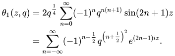


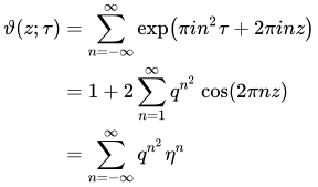








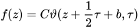



![{\displaystyle {\begin{aligned}\vartheta _{01}(z;\tau )&=\vartheta \left(z+{\tfrac {1}{2}};\tau \right)\\[3pt]\vartheta _{10}(z;\tau )&=\exp \left({\tfrac {1}{4}}\pi i\tau +\pi iz\right)\vartheta \left(z+{\tfrac {1}{2}}\tau ;\tau \right)\\[3pt]\vartheta _{11}(z;\tau )&=\exp \left({\tfrac {1}{4}}\pi i\tau +\pi i\left(z+{\tfrac {1}{2}}\right)\right)\vartheta \left(z+{\tfrac {1}{2}}\tau +{\tfrac {1}{2}};\tau \right).\end{aligned}}}](https://wikimedia.org/api/rest_v1/media/math/render/svg/ee051ca15813825e13589298c0efd02e3f68e0cf)


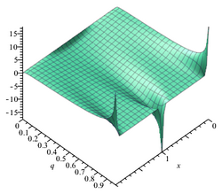

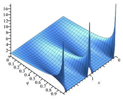


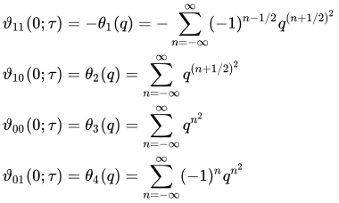


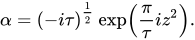
![{\displaystyle {\begin{aligned}\vartheta _{00}\!\left({\frac {z}{\tau }};{\frac {-1}{\tau }}\right)&=\alpha \,\vartheta _{00}(z;\tau )\quad &\vartheta _{01}\!\left({\frac {z}{\tau }};{\frac {-1}{\tau }}\right)&=\alpha \,\vartheta _{10}(z;\tau )\\[3pt]\vartheta _{10}\!\left({\frac {z}{\tau }};{\frac {-1}{\tau }}\right)&=\alpha \,\vartheta _{01}(z;\tau )\quad &\vartheta _{11}\!\left({\frac {z}{\tau }};{\frac {-1}{\tau }}\right)&=-i\alpha \,\vartheta _{11}(z;\tau ).\end{aligned}}}](https://wikimedia.org/api/rest_v1/media/math/render/svg/e38521d263e968c6643113cb856744c3d8417638)
![{\displaystyle {\begin{aligned}\vartheta _{00}(w,q)&=\sum _{n=-\infty }^{\infty }\left(w^{2}\right)^{n}q^{n^{2}}\quad &\vartheta _{01}(w,q)&=\sum _{n=-\infty }^{\infty }(-1)^{n}\left(w^{2}\right)^{n}q^{n^{2}}\\[3pt]\vartheta _{10}(w,q)&=\sum _{n=-\infty }^{\infty }\left(w^{2}\right)^{n+{\frac {1}{2}}}q^{\left(n+{\frac {1}{2}}\right)^{2}}\quad &\vartheta _{11}(w,q)&=i\sum _{n=-\infty }^{\infty }(-1)^{n}\left(w^{2}\right)^{n+{\frac {1}{2}}}q^{\left(n+{\frac {1}{2}}\right)^{2}}.\end{aligned}}}](https://wikimedia.org/api/rest_v1/media/math/render/svg/acbc490b1dd786cc2ef221b6b0834661d3f41ac3)



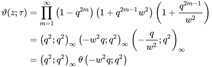


![{\displaystyle {\begin{aligned}\vartheta _{01}(z\mid q)&=\prod _{m=1}^{\infty }\left(1-q^{2m}\right)\left(1-2\cos(2\pi z)q^{2m-1}+q^{4m-2}\right),\\[3pt]\vartheta _{10}(z\mid q)&=2q^{\frac {1}{4}}\cos(\pi z)\prod _{m=1}^{\infty }\left(1-q^{2m}\right)\left(1+2\cos(2\pi z)q^{2m}+q^{4m}\right),\\[3pt]\vartheta _{11}(z\mid q)&=-2q^{\frac {1}{4}}\sin(\pi z)\prod _{m=1}^{\infty }\left(1-q^{2m}\right)\left(1-2\cos(2\pi z)q^{2m}+q^{4m}\right).\end{aligned}}}](https://wikimedia.org/api/rest_v1/media/math/render/svg/1a2f486ca65bf1df31851e9591220ff601cf6fb0)


![{\displaystyle {\begin{aligned}\vartheta _{00}(z;\tau )&=-i\int _{i-\infty }^{i+\infty }e^{i\pi \tau u^{2}}{\frac {\cos(2\pi uz+\pi u)}{\sin(\pi u)}}\mathrm {d} u;\\[6pt]\vartheta _{01}(z;\tau )&=-i\int _{i-\infty }^{i+\infty }e^{i\pi \tau u^{2}}{\frac {\cos(2\pi uz)}{\sin(\pi u)}}\mathrm {d} u;\\[6pt]\vartheta _{10}(z;\tau )&=-ie^{i\pi z+{\frac {1}{4}}i\pi \tau }\int _{i-\infty }^{i+\infty }e^{i\pi \tau u^{2}}{\frac {\cos(2\pi uz+\pi u+\pi \tau u)}{\sin(\pi u)}}\mathrm {d} u;\\[6pt]\vartheta _{11}(z;\tau )&=e^{i\pi z+{\frac {1}{4}}i\pi \tau }\int _{i-\infty }^{i+\infty }e^{i\pi \tau u^{2}}{\frac {\cos(2\pi uz+\pi \tau u)}{\sin(\pi u)}}\mathrm {d} u.\end{aligned}}}](https://wikimedia.org/api/rest_v1/media/math/render/svg/bd32c29ab16bda39187ec29c1169e8019bcb54af)

![{\displaystyle \theta _{3}(q)=1+{\frac {4q{\sqrt {\ln(1/q)}}}{\sqrt {\pi }}}\int _{0}^{\infty }{\frac {\exp[-\ln(1/q)\,x^{2}]\{1-q^{2}\cos[2\ln(1/q)\,x]\}}{1-2q^{2}\cos[2\ln(1/q)\,x]+q^{4}}}\,\mathrm {d} x}](https://wikimedia.org/api/rest_v1/media/math/render/svg/9e26186736a2e273adfa2732fea7ee65263231d4)
![{\displaystyle {\biggl [}{\frac {2}{\pi }}K{\bigl (}{\frac {1}{2}}{\sqrt {2}}{\bigr )}{\biggr ]}^{1/2}=\theta _{3}{\bigl [}\exp(-\pi ){\bigr ]}=1+4\exp(-\pi )\int _{0}^{\infty }{\frac {\exp(-\pi x^{2})[1-\exp(-2\pi )\cos(2\pi x)]}{1-2\exp(-2\pi )\cos(2\pi x)+\exp(-4\pi )}}\,\mathrm {d} x}](https://wikimedia.org/api/rest_v1/media/math/render/svg/942b823ba5f2a5d89016b6493ca9cc3b187cb86f)
![{\displaystyle {\biggl [}{\frac {2}{\pi }}K({\sqrt {2}}-1){\biggr ]}^{1/2}=\theta _{3}{\bigl [}\exp(-{\sqrt {2}}\,\pi ){\bigr ]}=1+4\,{\sqrt[{4}]{2}}\exp(-{\sqrt {2}}\,\pi )\int _{0}^{\infty }{\frac {\exp(-{\sqrt {2}}\,\pi x^{2})[1-\exp(-2{\sqrt {2}}\,\pi )\cos(2{\sqrt {2}}\,\pi x)]}{1-2\exp(-2{\sqrt {2}}\,\pi )\cos(2{\sqrt {2}}\,\pi x)+\exp(-4{\sqrt {2}}\,\pi )}}\,\mathrm {d} x}](https://wikimedia.org/api/rest_v1/media/math/render/svg/5cc3a6cd1621989208f56af90722f5230eecf7b6)
![{\displaystyle {\biggl \{}{\frac {2}{\pi }}K{\bigl [}\sin {\bigl (}{\frac {\pi }{12}}{\bigr )}{\bigr ]}{\biggr \}}^{1/2}=\theta _{3}{\bigl [}\exp(-{\sqrt {3}}\,\pi ){\bigr ]}=1+4\,{\sqrt[{4}]{3}}\exp(-{\sqrt {3}}\,\pi )\int _{0}^{\infty }{\frac {\exp(-{\sqrt {3}}\,\pi x^{2})[1-\exp(-2{\sqrt {3}}\,\pi )\cos(2{\sqrt {3}}\,\pi x)]}{1-2\exp(-2{\sqrt {3}}\,\pi )\cos(2{\sqrt {3}}\,\pi x)+\exp(-4{\sqrt {3}}\,\pi )}}\,\mathrm {d} x}](https://wikimedia.org/api/rest_v1/media/math/render/svg/9d462b60e5965c30acaf2837ae9770eb3a3560f5)


![{\displaystyle \theta _{3}\left({\frac {1}{2}}\right)=1+2\sum _{n=1}^{\infty }{\frac {1}{2^{n^{2}}}}=1+2\pi ^{-1/2}{\sqrt {\ln(2)}}\int _{0}^{\infty }{\frac {\exp[-\ln(2)\,x^{2}]\{16-4\cos[2\ln(2)\,x]\}}{17-8\cos[2\ln(2)\,x]}}\,\mathrm {d} x}](https://wikimedia.org/api/rest_v1/media/math/render/svg/80285f837f55ecc6e8a2d0b82edd47eb6a50467b)

![{\displaystyle \theta _{3}\left({\frac {1}{3}}\right)=1+2\sum _{n=1}^{\infty }{\frac {1}{3^{n^{2}}}}=1+{\frac {4}{3}}\pi ^{-1/2}{\sqrt {\ln(3)}}\int _{0}^{\infty }{\frac {\exp[-\ln(3)\,x^{2}]\{81-9\cos[2\ln(3)\,x]\}}{82-18\cos[2\ln(3)\,x]}}\,\mathrm {d} x}](https://wikimedia.org/api/rest_v1/media/math/render/svg/b778736b39bddab58af391077803cffab7928c6c)





![{\displaystyle {\begin{aligned}\varphi \left(e^{-\pi }\right)&={\frac {\sqrt[{4}]{\pi }}{\Gamma \left({\frac {3}{4}}\right)}}={\sqrt {2}}\,\eta \left({\sqrt {-1}}\right)\\\varphi \left(e^{-2\pi }\right)&={\frac {\sqrt[{4}]{\pi }}{\Gamma \left({\frac {3}{4}}\right)}}{\frac {\sqrt {2+{\sqrt {2}}}}{2}}\\\varphi \left(e^{-3\pi }\right)&={\frac {\sqrt[{4}]{\pi }}{\Gamma \left({\frac {3}{4}}\right)}}{\frac {\sqrt {1+{\sqrt {3}}}}{\sqrt[{8}]{108}}}\\\varphi \left(e^{-4\pi }\right)&={\frac {\sqrt[{4}]{\pi }}{\Gamma \left({\frac {3}{4}}\right)}}{\frac {2+{\sqrt[{4}]{8}}}{4}}\\\varphi \left(e^{-5\pi }\right)&={\frac {\sqrt[{4}]{\pi }}{\Gamma \left({\frac {3}{4}}\right)}}{\sqrt {\frac {2+{\sqrt {5}}}{5}}}\\\varphi \left(e^{-6\pi }\right)&={\frac {\sqrt[{4}]{\pi }}{\Gamma \left({\frac {3}{4}}\right)}}{\frac {\sqrt {{\sqrt[{4}]{1}}+{\sqrt[{4}]{3}}+{\sqrt[{4}]{4}}+{\sqrt[{4}]{9}}}}{\sqrt[{8}]{12^{3}}}}\\\varphi \left(e^{-7\pi }\right)&={\frac {\sqrt[{4}]{\pi }}{\Gamma \left({\frac {3}{4}}\right)}}{\frac {\sqrt {{\sqrt {13+{\sqrt {7}}}}+{\sqrt {7+3{\sqrt {7}}}}}}{{\sqrt[{8}]{14^{3}}}\cdot {\sqrt[{16}]{7}}}}\\\varphi \left(e^{-8\pi }\right)&={\frac {\sqrt[{4}]{\pi }}{\Gamma \left({\frac {3}{4}}\right)}}{\frac {{\sqrt {2+{\sqrt {2}}}}+{\sqrt[{8}]{128}}}{4}}\\\varphi \left(e^{-9\pi }\right)&={\frac {\sqrt[{4}]{\pi }}{\Gamma \left({\frac {3}{4}}\right)}}{\frac {1+{\sqrt[{3}]{2+2{\sqrt {3}}}}}{3}}\\\varphi \left(e^{-10\pi }\right)&={\frac {\sqrt[{4}]{\pi }}{\Gamma \left({\frac {3}{4}}\right)}}{\frac {\sqrt {{\sqrt[{4}]{64}}+{\sqrt[{4}]{80}}+{\sqrt[{4}]{81}}+{\sqrt[{4}]{100}}}}{\sqrt[{4}]{200}}}\\\varphi \left(e^{-11\pi }\right)&={\frac {\sqrt[{4}]{\pi }}{\Gamma \left({\frac {3}{4}}\right)}}{\frac {\sqrt {11+{\sqrt {11}}+(5+3{\sqrt {3}}+{\sqrt {11}}+{\sqrt {33}}){\sqrt[{3}]{-44+33{\sqrt {3}}}}+(-5+3{\sqrt {3}}-{\sqrt {11}}+{\sqrt {33}}){\sqrt[{3}]{44+33{\sqrt {3}}}}}}{\sqrt[{8}]{52180524}}}\\\varphi \left(e^{-12\pi }\right)&={\frac {\sqrt[{4}]{\pi }}{\Gamma \left({\frac {3}{4}}\right)}}{\frac {\sqrt {{\sqrt[{4}]{1}}+{\sqrt[{4}]{2}}+{\sqrt[{4}]{3}}+{\sqrt[{4}]{4}}+{\sqrt[{4}]{9}}+{\sqrt[{4}]{18}}+{\sqrt[{4}]{24}}}}{2{\sqrt[{8}]{108}}}}\\\varphi \left(e^{-13\pi }\right)&={\frac {\sqrt[{4}]{\pi }}{\Gamma \left({\frac {3}{4}}\right)}}{\frac {\sqrt {13+8{\sqrt {13}}+(11-6{\sqrt {3}}+{\sqrt {13}}){\sqrt[{3}]{143+78{\sqrt {3}}}}+(11+6{\sqrt {3}}+{\sqrt {13}}){\sqrt[{3}]{143-78{\sqrt {3}}}}}}{\sqrt[{4}]{19773}}}\\\varphi \left(e^{-14\pi }\right)&={\frac {\sqrt[{4}]{\pi }}{\Gamma \left({\frac {3}{4}}\right)}}{\frac {\sqrt {{\sqrt {13+{\sqrt {7}}}}+{\sqrt {7+3{\sqrt {7}}}}+{\sqrt {10+2{\sqrt {7}}}}+{\sqrt[{8}]{28}}{\sqrt {4+{\sqrt {7}}}}}}{\sqrt[{16}]{28^{7}}}}\\\varphi \left(e^{-15\pi }\right)&={\frac {\sqrt[{4}]{\pi }}{\Gamma \left({\frac {3}{4}}\right)}}{\frac {\sqrt {7+3{\sqrt {3}}+{\sqrt {5}}+{\sqrt {15}}+{\sqrt[{4}]{60}}+{\sqrt[{4}]{1500}}}}{{\sqrt[{8}]{12^{3}}}\cdot {\sqrt {5}}}}\\2\varphi \left(e^{-16\pi }\right)&=\varphi \left(e^{-4\pi }\right)+{\frac {\sqrt[{4}]{\pi }}{\Gamma \left({\frac {3}{4}}\right)}}{\frac {\sqrt[{4}]{1+{\sqrt {2}}}}{\sqrt[{16}]{128}}}\\\varphi \left(e^{-17\pi }\right)&={\frac {\sqrt[{4}]{\pi }}{\Gamma \left({\frac {3}{4}}\right)}}{\frac {{\sqrt {2}}(1+{\sqrt[{4}]{17}})+{\sqrt[{8}]{17}}{\sqrt {5+{\sqrt {17}}}}}{\sqrt {17+17{\sqrt {17}}}}}\\2\varphi \left(e^{-20\pi }\right)&=\varphi \left(e^{-5\pi }\right)+{\frac {\sqrt[{4}]{\pi }}{\Gamma \left({\frac {3}{4}}\right)}}{\sqrt {\frac {3+2{\sqrt[{4}]{5}}}{5{\sqrt {2}}}}}\\6\varphi \left(e^{-36\pi }\right)&=3\varphi \left(e^{-9\pi }\right)+2\varphi \left(e^{-4\pi }\right)-\varphi \left(e^{-\pi }\right)+{\frac {\sqrt[{4}]{\pi }}{\Gamma \left({\frac {3}{4}}\right)}}{\sqrt[{3}]{{\sqrt[{4}]{2}}+{\sqrt[{4}]{18}}+{\sqrt[{4}]{216}}}}\end{aligned}}}](https://wikimedia.org/api/rest_v1/media/math/render/svg/d06e5700e306ee31cbf5d9565847590b4d4b966a)


![{\displaystyle \varphi {\bigl [}\exp(-{\tfrac {1}{5}}\pi ){\bigr ]}={\sqrt[{4}]{\pi }}\,{\Gamma \left({\tfrac {3}{4}}\right)}^{-1}\operatorname {slh} {\bigl (}{\tfrac {1}{5}}{\sqrt {2}}\,\varpi {\bigr )}\operatorname {slh} {\bigl (}{\tfrac {2}{5}}{\sqrt {2}}\,\varpi {\bigr )}}](https://wikimedia.org/api/rest_v1/media/math/render/svg/087f2996a1cad31a875a6346e7b52be98453668f)
![{\displaystyle \varphi {\bigl [}\exp(-{\tfrac {1}{7}}\pi ){\bigr ]}={\sqrt[{4}]{\pi }}\,{\Gamma \left({\tfrac {3}{4}}\right)}^{-1}\operatorname {slh} {\bigl (}{\tfrac {1}{7}}{\sqrt {2}}\,\varpi {\bigr )}\operatorname {slh} {\bigl (}{\tfrac {2}{7}}{\sqrt {2}}\,\varpi {\bigr )}\operatorname {slh} {\bigl (}{\tfrac {3}{7}}{\sqrt {2}}\,\varpi {\bigr )}}](https://wikimedia.org/api/rest_v1/media/math/render/svg/f01f0cb2fd209abfbb1ac4c204c509f2b3f47b74)
![{\displaystyle \varphi {\bigl [}\exp(-{\tfrac {1}{9}}\pi ){\bigr ]}={\sqrt[{4}]{\pi }}\,{\Gamma \left({\tfrac {3}{4}}\right)}^{-1}\operatorname {slh} {\bigl (}{\tfrac {1}{9}}{\sqrt {2}}\,\varpi {\bigr )}\operatorname {slh} {\bigl (}{\tfrac {2}{9}}{\sqrt {2}}\,\varpi {\bigr )}\operatorname {slh} {\bigl (}{\tfrac {3}{9}}{\sqrt {2}}\,\varpi {\bigr )}\operatorname {slh} {\bigl (}{\tfrac {4}{9}}{\sqrt {2}}\,\varpi {\bigr )}}](https://wikimedia.org/api/rest_v1/media/math/render/svg/51aea624bd4ccfed27077389532d4b07efda771e)
![{\displaystyle \varphi {\bigl [}\exp(-{\tfrac {1}{11}}\pi ){\bigr ]}={\sqrt[{4}]{\pi }}\,{\Gamma \left({\tfrac {3}{4}}\right)}^{-1}\operatorname {slh} {\bigl (}{\tfrac {1}{11}}{\sqrt {2}}\,\varpi {\bigr )}\operatorname {slh} {\bigl (}{\tfrac {2}{11}}{\sqrt {2}}\,\varpi {\bigr )}\operatorname {slh} {\bigl (}{\tfrac {3}{11}}{\sqrt {2}}\,\varpi {\bigr )}\operatorname {slh} {\bigl (}{\tfrac {4}{11}}{\sqrt {2}}\,\varpi {\bigr )}\operatorname {slh} {\bigl (}{\tfrac {5}{11}}{\sqrt {2}}\,\varpi {\bigr )}}](https://wikimedia.org/api/rest_v1/media/math/render/svg/3839f652515fbc383f7fa265b6541beaa7582c59)

![{\displaystyle {\begin{aligned}2\varphi \left(q^{4}\right)&=\varphi (q)+{\sqrt {2\varphi ^{2}\left(q^{2}\right)-\varphi ^{2}(q)}}\\3\varphi \left(q^{9}\right)&=\varphi (q)+{\sqrt[{3}]{9{\frac {\varphi ^{4}\left(q^{3}\right)}{\varphi (q)}}-\varphi ^{3}(q)}}\\{\sqrt {5}}\varphi \left(q^{25}\right)&=\varphi \left(q^{5}\right)\cot \left({\frac {1}{2}}\arctan \left({\frac {2}{\sqrt {5}}}{\frac {\varphi (q)\varphi \left(q^{5}\right)}{\varphi ^{2}(q)-\varphi ^{2}\left(q^{5}\right)}}{\frac {1+s(q)-s^{2}(q)}{s(q)}}\right)\right)\end{aligned}}}](https://wikimedia.org/api/rest_v1/media/math/render/svg/e3a018fbcd1409ba1ebb0c85d8178fb163fa3ba0)

![{\displaystyle {\begin{aligned}s(q)&={\sqrt[{5}]{\tan \left({\frac {1}{2}}\arctan \left({\frac {5}{2}}{\frac {\varphi ^{2}\left(q^{5}\right)}{\varphi ^{2}(q)}}-{\frac {1}{2}}\right)\right)\cot ^{2}\left({\frac {1}{2}}\operatorname {arccot} \left({\frac {5}{2}}{\frac {\varphi ^{2}\left(q^{5}\right)}{\varphi ^{2}(q)}}-{\frac {1}{2}}\right)\right)}}\\&={\cfrac {e^{-\pi i/(25\tau )}}{1-{\cfrac {e^{-\pi i/(5\tau )}}{1+{\cfrac {e^{-2\pi i/(5\tau )}}{1-\ddots }}}}}}\end{aligned}}}](https://wikimedia.org/api/rest_v1/media/math/render/svg/de23ddbf5b96a5a2470d73ba10f05153d2a7e37d)
![{\displaystyle {\begin{array}{lll}\varphi \left(\exp(-{\sqrt {3}}\,\pi )\right)&=&\pi ^{-1}{\Gamma \left({\tfrac {4}{3}}\right)}^{3/2}2^{-2/3}3^{13/8}\\\varphi \left(\exp(-2{\sqrt {3}}\,\pi )\right)&=&\pi ^{-1}{\Gamma \left({\tfrac {4}{3}}\right)}^{3/2}2^{-2/3}3^{13/8}\cos({\tfrac {1}{24}}\pi )\\\varphi \left(\exp(-3{\sqrt {3}}\,\pi )\right)&=&\pi ^{-1}{\Gamma \left({\tfrac {4}{3}}\right)}^{3/2}2^{-2/3}3^{7/8}({\sqrt[{3}]{2}}+1)\\\varphi \left(\exp(-4{\sqrt {3}}\,\pi )\right)&=&\pi ^{-1}{\Gamma \left({\tfrac {4}{3}}\right)}^{3/2}2^{-5/3}3^{13/8}{\Bigl (}1+{\sqrt {\cos({\tfrac {1}{12}}\pi )}}{\Bigr )}\\\varphi \left(\exp(-5{\sqrt {3}}\,\pi )\right)&=&\pi ^{-1}{\Gamma \left({\tfrac {4}{3}}\right)}^{3/2}2^{-2/3}3^{5/8}\sin({\tfrac {1}{5}}\pi )({\tfrac {2}{5}}{\sqrt[{3}]{100}}+{\tfrac {2}{5}}{\sqrt[{3}]{10}}+{\tfrac {3}{5}}{\sqrt {5}}+1)\end{array}}}](https://wikimedia.org/api/rest_v1/media/math/render/svg/913e0c2a4e7f8efd215821d4423789caf3cc7382)
![{\displaystyle \theta _{2}(q^{2})={\tfrac {1}{2}}{\sqrt {2[\theta _{3}(q)^{2}-\theta _{4}(q)^{2}]}}}](https://wikimedia.org/api/rest_v1/media/math/render/svg/49fdbf249a5c77891ea7be62a7abdb74bfca9c20)
![{\displaystyle \theta _{3}(q^{2})={\tfrac {1}{2}}{\sqrt {2[\theta _{3}(q)^{2}+\theta _{4}(q)^{2}]}}}](https://wikimedia.org/api/rest_v1/media/math/render/svg/ab78a4868b53c96cb965bc889ba12f8e4fd5bd44)
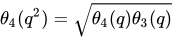

![{\displaystyle 27\,\theta _{3}(q^{3})^{8}-18\,\theta _{3}(q^{3})^{4}\theta _{3}(q)^{4}-\,\theta _{3}(q)^{8}=8\,\theta _{3}(q^{3})^{2}\theta _{3}(q)^{2}[2\,\theta _{4}(q)^{4}-\theta _{3}(q)^{4}]}](https://wikimedia.org/api/rest_v1/media/math/render/svg/ee8b22b2491acbf41acf156847592744fe5efda4)
![{\displaystyle 27\,\theta _{4}(q^{3})^{8}-18\,\theta _{4}(q^{3})^{4}\theta _{4}(q)^{4}-\,\theta _{4}(q)^{8}=8\,\theta _{4}(q^{3})^{2}\theta _{4}(q)^{2}[2\,\theta _{3}(q)^{4}-\theta _{4}(q)^{4}]}](https://wikimedia.org/api/rest_v1/media/math/render/svg/6db22a825f23c8747194677df1ba5b9cd6776c58)
![{\displaystyle [\theta _{3}(q)^{2}-\theta _{3}(q^{5})^{2}][5\,\theta _{3}(q^{5})^{2}-\theta _{3}(q)^{2}]^{5}=256\,\theta _{3}(q^{5})^{2}\theta _{3}(q)^{2}\theta _{4}(q)^{4}[\theta _{3}(q)^{4}-\theta _{4}(q)^{4}]}](https://wikimedia.org/api/rest_v1/media/math/render/svg/21698abd5cd7e4f2b57023ecd5dd70b3fd545ffb)
![{\displaystyle [\theta _{4}(q^{5})^{2}-\theta _{4}(q)^{2}][5\,\theta _{4}(q^{5})^{2}-\theta _{4}(q)^{2}]^{5}=256\,\theta _{4}(q^{5})^{2}\theta _{4}(q)^{2}\theta _{3}(q)^{4}[\theta _{3}(q)^{4}-\theta _{4}(q)^{4}]}](https://wikimedia.org/api/rest_v1/media/math/render/svg/6bc5563a31bcb890a22ebb282ad224297a82b287)
![{\displaystyle {\biggl [}{\frac {\theta _{3}(q^{1/3})^{2}}{\theta _{3}(q)^{2}}}-{\frac {3\,\theta _{3}(q^{3})^{2}}{\theta _{3}(q)^{2}}}{\biggr ]}^{2}=4-4{\biggl [}{\frac {2\,\theta _{2}(q)^{2}\theta _{4}(q)^{2}}{\theta _{3}(q)^{4}}}{\biggr ]}^{2/3}}](https://wikimedia.org/api/rest_v1/media/math/render/svg/a41eb7bba4644993c0994d693977d751526d68a1)
![{\displaystyle {\biggl [}{\frac {3\,\theta _{4}(q^{3})^{2}}{\theta _{4}(q)^{2}}}-{\frac {\theta _{4}(q^{1/3})^{2}}{\theta _{4}(q)^{2}}}{\biggr ]}^{2}=4+4{\biggl [}{\frac {2\,\theta _{2}(q)^{2}\theta _{3}(q)^{2}}{\theta _{4}(q)^{4}}}{\biggr ]}^{2/3}}](https://wikimedia.org/api/rest_v1/media/math/render/svg/f4d0741127e031b7079dffa001160094eb9b03c9)
![{\displaystyle R(q)=\tan {\biggl \{}{\frac {1}{2}}\arctan {\biggl [}{\frac {1}{2}}-{\frac {\theta _{4}(q)^{2}}{2\,\theta _{4}(q^{5})^{2}}}{\biggr ]}{\biggr \}}^{1/5}\tan {\biggl \{}{\frac {1}{2}}\operatorname {arccot} {\biggl [}{\frac {1}{2}}-{\frac {\theta _{4}(q)^{2}}{2\,\theta _{4}(q^{5})^{2}}}{\biggr ]}{\biggr \}}^{2/5}}](https://wikimedia.org/api/rest_v1/media/math/render/svg/122911c8d5591255a99de086a6643e60e8496af8)
![{\displaystyle R(q^{2})=\tan {\biggl \{}{\frac {1}{2}}\arctan {\biggl [}{\frac {1}{2}}-{\frac {\theta _{4}(q)^{2}}{2\,\theta _{4}(q^{5})^{2}}}{\biggr ]}{\biggr \}}^{2/5}\cot {\biggl \{}{\frac {1}{2}}\operatorname {arccot} {\biggl [}{\frac {1}{2}}-{\frac {\theta _{4}(q)^{2}}{2\,\theta _{4}(q^{5})^{2}}}{\biggr ]}{\biggr \}}^{1/5}}](https://wikimedia.org/api/rest_v1/media/math/render/svg/87bef51d2716d70a8054cd882a9c6a98aa234b16)
![{\displaystyle R(q^{2})=\tan {\biggl \{}{\frac {1}{2}}\arctan {\biggl [}{\frac {\theta _{3}(q)^{2}}{2\,\theta _{3}(q^{5})^{2}}}-{\frac {1}{2}}{\biggr ]}{\biggr \}}^{2/5}\tan {\biggl \{}{\frac {1}{2}}\operatorname {arccot} {\biggl [}{\frac {\theta _{3}(q)^{2}}{2\,\theta _{3}(q^{5})^{2}}}-{\frac {1}{2}}{\biggr ]}{\biggr \}}^{1/5}}](https://wikimedia.org/api/rest_v1/media/math/render/svg/6fd8befdabb6ac82b6c4fff8f0a5bb89a1a5ac55)
![{\displaystyle S(q)={\frac {R(q^{4})}{R(q^{2})R(q)}}=\tan {\biggl \{}{\frac {1}{2}}\arctan {\biggl [}{\frac {\theta _{3}(q)^{2}}{2\,\theta _{3}(q^{5})^{2}}}-{\frac {1}{2}}{\biggr ]}{\biggr \}}^{1/5}\cot {\biggl \{}{\frac {1}{2}}\operatorname {arccot} {\biggl [}{\frac {\theta _{3}(q)^{2}}{2\,\theta _{3}(q^{5})^{2}}}-{\frac {1}{2}}{\biggr ]}{\biggr \}}^{2/5}}](https://wikimedia.org/api/rest_v1/media/math/render/svg/968499610c12ca2700607ba9048ff01e2f8fe303)
![{\displaystyle {\frac {\theta _{3}(q^{1/5})}{\theta _{3}(q^{5})}}-1={\frac {1}{S(q)}}{\bigl [}S(q)^{2}+R(q^{2}){\bigr ]}{\bigl [}1+R(q^{2})S(q){\bigr ]}}](https://wikimedia.org/api/rest_v1/media/math/render/svg/3e1f9826acfe6b0205eb7dec745ce83aae7e6d01)
![{\displaystyle 1-{\frac {\theta _{4}(q^{1/5})}{\theta _{4}(q^{5})}}={\frac {1}{R(q)}}{\bigl [}R(q^{2})+R(q)^{2}{\bigr ]}{\bigl [}1-R(q^{2})R(q){\bigr ]}}](https://wikimedia.org/api/rest_v1/media/math/render/svg/cb6fd08483ead704a199a261edcf54d483835ad9)
![{\displaystyle \theta _{3}(q^{1/5})^{2}-\theta _{3}(q)^{2}={\bigl [}\theta _{3}(q)^{2}-\theta _{3}(q^{5})^{2}{\bigr ]}{\biggl [}1+{\frac {1}{R(q^{2})S(q)}}+R(q^{2})S(q)+{\frac {1}{R(q^{2})^{2}}}+R(q^{2})^{2}+{\frac {1}{S(q)}}-S(q){\biggr ]}}](https://wikimedia.org/api/rest_v1/media/math/render/svg/c87e7c0cdbc5280e1ca49f87d77c2924e364d6c6)
![{\displaystyle \theta _{4}(q)^{2}-\theta _{4}(q^{1/5})^{2}={\bigl [}\theta _{4}(q^{5})^{2}-\theta _{4}(q)^{2}{\bigr ]}{\biggl [}1-{\frac {1}{R(q^{2})R(q)}}-R(q^{2})R(q)+{\frac {1}{R(q^{2})^{2}}}+R(q^{2})^{2}-{\frac {1}{R(q)}}+R(q){\biggr ]}}](https://wikimedia.org/api/rest_v1/media/math/render/svg/6e4601790cf31b8e82943713c410b532e4d75980)
![{\displaystyle \theta _{4}[q(k)]=\theta _{4}[q(k)^{2}]{\sqrt[{8}]{1-k^{2}}}}](https://wikimedia.org/api/rest_v1/media/math/render/svg/ece5e6b2598db08419e115b84fa8dc058e3980b8)
![{\displaystyle \theta _{4}[q(k)^{2}]=\theta _{3}[q(k)]{\sqrt[{8}]{1-k^{2}}}}](https://wikimedia.org/api/rest_v1/media/math/render/svg/85cc179f3c7fab7e4f664ea3a9ad3bed2c751a65)
![{\displaystyle \theta _{3}[q(k)^{2}]=\theta _{3}[q(k)]\cos[{\tfrac {1}{2}}\arcsin(k)]}](https://wikimedia.org/api/rest_v1/media/math/render/svg/9a0b0e95b8b6fd152fc74a01c0f7fbab2b9a6555)
![{\displaystyle \theta _{4}{\biggl \langle }q{\bigl \{}\tan {\bigl [}{\tfrac {1}{2}}\arctan(t^{3}){\bigr ]}{\bigr \}}^{3}{\biggr \rangle }=\theta _{4}{\biggl \langle }q{\bigl \{}\tan {\bigl [}{\tfrac {1}{2}}\arctan(t^{3}){\bigr ]}{\bigr \}}{\biggr \rangle }\,3^{-1/2}{\bigl (}{\sqrt {2{\sqrt {t^{4}-t^{2}+1}}-t^{2}+2}}+{\sqrt {t^{2}+1}}\,{\bigr )}^{1/2}}](https://wikimedia.org/api/rest_v1/media/math/render/svg/0608e409cfd0018afa26a9e4561bc8ce04b7c964)


![{\displaystyle \theta _{4}{\biggl \langle }q{\bigl \{}\tan {\bigl [}{\tfrac {1}{2}}\arctan(1){\bigr ]}{\bigr \}}^{3}{\biggr \rangle }=\theta _{4}{\biggl \langle }q{\bigl \{}\tan {\bigl [}{\tfrac {1}{2}}\arctan(1){\bigr ]}{\bigr \}}{\biggr \rangle }\,3^{-1/2}{\bigl (}{\sqrt {3}}+{\sqrt {2}}\,{\bigr )}^{1/2}}](https://wikimedia.org/api/rest_v1/media/math/render/svg/27d9399dd8871346e454374d0965a18caba1db5c)
![{\displaystyle \theta _{4}{\bigl [}\exp(-3{\sqrt {2}}\,\pi ){\bigr ]}=\theta _{4}{\bigl [}\exp(-{\sqrt {2}}\,\pi ){\bigr ]}\,3^{-1/2}{\bigl (}{\sqrt {3}}+{\sqrt {2}}\,{\bigr )}^{1/2}}](https://wikimedia.org/api/rest_v1/media/math/render/svg/d24c901354972a0b0861ecf1304c11b74666f25b)

![{\displaystyle \theta _{4}{\biggl \langle }q{\bigl \{}\tan {\bigl [}{\tfrac {1}{2}}\arctan(\Phi ^{-6}){\bigr ]}{\bigr \}}^{3}{\biggr \rangle }=\theta _{4}{\biggl \langle }q{\bigl \{}\tan {\bigl [}{\tfrac {1}{2}}\arctan(\Phi ^{-6}){\bigr ]}{\bigr \}}{\biggr \rangle }\,3^{-1/2}{\bigl (}{\sqrt {2{\sqrt {\Phi ^{-8}-\Phi ^{-4}+1}}-\Phi ^{-4}+2}}+{\sqrt {\Phi ^{-4}+1}}\,{\bigr )}^{1/2}}](https://wikimedia.org/api/rest_v1/media/math/render/svg/7dc07d14cd349f46b4f18689ce8fc44277e67902)
![{\displaystyle \theta _{4}{\bigl [}\exp(-3{\sqrt {10}}\,\pi ){\bigr ]}=\theta _{4}{\bigl [}\exp(-{\sqrt {10}}\,\pi ){\bigr ]}\,3^{-1/2}{\bigl (}{\sqrt {2{\sqrt {\Phi ^{-8}-\Phi ^{-4}+1}}-\Phi ^{-4}+2}}+{\sqrt {\Phi ^{-4}+1}}\,{\bigr )}^{1/2}}](https://wikimedia.org/api/rest_v1/media/math/render/svg/76245ff2f6bee7a43882f3f4ebbcad691b406a96)

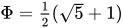

![{\displaystyle ={\frac {\sqrt {5}}{4}}\,\theta _{2}(\Phi ^{-2})^{2}={\frac {\sqrt {5}}{8}}{\bigl [}\theta _{3}(\Phi ^{-1})^{2}-\theta _{4}(\Phi ^{-1})^{2}{\bigr ]}}](https://wikimedia.org/api/rest_v1/media/math/render/svg/e05e65a1d4c792ec63055ed7d1d9a08f7faf285e)
![{\displaystyle \sum _{n=1}^{\infty }{\frac {1}{F_{2n-1}}}={\frac {\sqrt {5}}{4}}\,{\biggl [}\sum _{n=1}^{\infty }2\,\Phi ^{-(2n-1)^{2}/2}{\biggr ]}^{2}}](https://wikimedia.org/api/rest_v1/media/math/render/svg/e0218550f8623ef9dce9705bde847639ee6e6919)

![{\displaystyle \sum _{n=1}^{\infty }{\frac {1}{F_{n}^{2}}}={\frac {5}{24}}{\bigl [}2\,\theta _{2}(\Phi ^{-2})^{4}-\theta _{3}(\Phi ^{-2})^{4}+1{\bigr ]}={\frac {5}{24}}{\bigl [}\theta _{3}(\Phi ^{-2})^{4}-2\,\theta _{4}(\Phi ^{-2})^{4}+1{\bigr ]}}](https://wikimedia.org/api/rest_v1/media/math/render/svg/71c7f301cb452442a43e1fcd9c91ea78bc820ef9)
![{\displaystyle \sum _{n=1}^{\infty }{\frac {1}{P_{2n-1}}}={\frac {1}{\sqrt {2}}}\,\theta _{2}{\bigl [}({\sqrt {2}}-1)^{2}{\bigr ]}^{2}={\frac {1}{2{\sqrt {2}}}}{\bigl [}\theta _{3}({\sqrt {2}}-1)^{2}-\theta _{4}({\sqrt {2}}-1)^{2}{\bigr ]}}](https://wikimedia.org/api/rest_v1/media/math/render/svg/25a2e2b5ff5d3f65182b77f5be772944bc4d6ea2)
![{\displaystyle {\begin{aligned}\theta _{4}^{2}(q)&=iq^{\frac {1}{4}}\sum _{k=-\infty }^{\infty }q^{2k^{2}-k}\theta _{1}\left({\frac {2k-1}{2i}}\ln q,q\right),\\[6pt]\theta _{4}^{2}(q)&=\sum _{k=-\infty }^{\infty }q^{2k^{2}}\theta _{4}\left({\frac {k\ln q}{i}},q\right).\end{aligned}}}](https://wikimedia.org/api/rest_v1/media/math/render/svg/428f8073ad45e4e54778db88a3dbb2f5b0ab1f30)

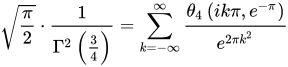
![{\displaystyle {\begin{aligned}\vartheta (z;\tau )=\vartheta _{00}(z;\tau )&=0\quad &\Longleftrightarrow &&\quad z&=m+n\tau +{\frac {1}{2}}+{\frac {\tau }{2}}\\[3pt]\vartheta _{11}(z;\tau )&=0\quad &\Longleftrightarrow &&\quad z&=m+n\tau \\[3pt]\vartheta _{10}(z;\tau )&=0\quad &\Longleftrightarrow &&\quad z&=m+n\tau +{\frac {1}{2}}\\[3pt]\vartheta _{01}(z;\tau )&=0\quad &\Longleftrightarrow &&\quad z&=m+n\tau +{\frac {\tau }{2}}\end{aligned}}}](https://wikimedia.org/api/rest_v1/media/math/render/svg/fcdb60358dddb241ffda786440efa91cc0844ca9)




![{\displaystyle {\begin{aligned}\theta _{2}(q)=\vartheta _{10}(0;\tau )&={\frac {2\eta ^{2}(2\tau )}{\eta (\tau )}},\\[3pt]\theta _{3}(q)=\vartheta _{00}(0;\tau )&={\frac {\eta ^{5}(\tau )}{\eta ^{2}\left({\frac {1}{2}}\tau \right)\eta ^{2}(2\tau )}}={\frac {\eta ^{2}\left({\frac {1}{2}}(\tau +1)\right)}{\eta (\tau +1)}},\\[3pt]\theta _{4}(q)=\vartheta _{01}(0;\tau )&={\frac {\eta ^{2}\left({\frac {1}{2}}\tau \right)}{\eta (\tau )}},\end{aligned}}}](https://wikimedia.org/api/rest_v1/media/math/render/svg/2358dd2d333a2740823f158700af932d247a2c7e)

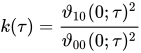
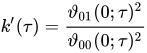

![{\displaystyle E(k)={\frac {\pi }{2}}\sum _{a=0}^{\infty }{\frac {[(2a)!]^{2}}{(1-2a)16^{a}(a!)^{4}}}k^{2a}}](https://wikimedia.org/api/rest_v1/media/math/render/svg/4a4e8c4e1616502c6de3e16bb661c1372b93c0fd)



![{\displaystyle \theta _{2}'(x)={\frac {\mathrm {d} }{\mathrm {d} x}}\,\theta _{2}(x)={\frac {1}{2\pi x}}\theta _{2}(x)\theta _{3}(x)^{2}E{\biggl [}{\frac {\theta _{2}(x)^{2}}{\theta _{3}(x)^{2}}}{\biggr ]}}](https://wikimedia.org/api/rest_v1/media/math/render/svg/0a311084c05bdae1b514737c2f0108933b9f8bae)
![{\displaystyle \theta _{3}'(x)={\frac {\mathrm {d} }{\mathrm {d} x}}\,\theta _{3}(x)=\theta _{3}(x){\bigl [}\theta _{3}(x)^{2}+\theta _{4}(x)^{2}{\bigr ]}{\biggl \{}{\frac {1}{2\pi x}}E{\biggl [}{\frac {\theta _{3}(x)^{2}-\theta _{4}(x)^{2}}{\theta _{3}(x)^{2}+\theta _{4}(x)^{2}}}{\biggr ]}-{\frac {\theta _{4}(x)^{2}}{4\,x}}{\biggr \}}}](https://wikimedia.org/api/rest_v1/media/math/render/svg/104d1b3737a0be4eda8a3a1e245186de9134a6e9)
![{\displaystyle \theta _{4}'(x)={\frac {\mathrm {d} }{\mathrm {d} x}}\,\theta _{4}(x)=\theta _{4}(x){\bigl [}\theta _{3}(x)^{2}+\theta _{4}(x)^{2}{\bigr ]}{\biggl \{}{\frac {1}{2\pi x}}E{\biggl [}{\frac {\theta _{3}(x)^{2}-\theta _{4}(x)^{2}}{\theta _{3}(x)^{2}+\theta _{4}(x)^{2}}}{\biggr ]}-{\frac {\theta _{3}(x)^{2}}{4\,x}}{\biggr \}}}](https://wikimedia.org/api/rest_v1/media/math/render/svg/2f5be9c018c56615a9085df89d3db2ca5d7d26b5)

![{\displaystyle \vartheta _{4}(x){\biggl [}{\frac {\mathrm {d} }{\mathrm {d} x}}\,\vartheta _{3}(x){\biggr ]}-\vartheta _{3}(x){\biggl [}{\frac {\mathrm {d} }{\mathrm {d} x}}\,\theta _{4}(x){\biggr ]}={\frac {1}{4\,x}}\,\theta _{3}(x)\,\theta _{4}(x){\bigl [}\theta _{3}(x)^{4}-\theta _{4}(x)^{4}{\bigr ]}}](https://wikimedia.org/api/rest_v1/media/math/render/svg/b88237a98911175d2efc60c4d21094300a862abd)
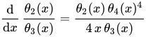
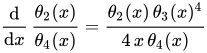





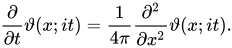
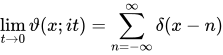


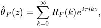
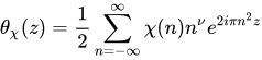
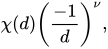
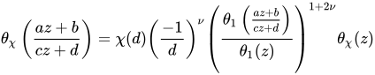











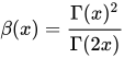

![{\displaystyle {\frac {4^{-1/(n+2)}}{n+2}}\csc {\bigl (}{\frac {\pi }{n+2}}{\bigr )}\beta {\biggl [}{\frac {n}{2(n+2)}}{\biggr ]}=\int _{0}^{\infty }{\frac {1}{\sqrt {x^{n+2}+1}}}\,\mathrm {d} x}](https://wikimedia.org/api/rest_v1/media/math/render/svg/48152e52c3eb9c14398e29907e759b53900153c6)
![{\displaystyle {\frac {1}{\sqrt {x^{4}+1}}}={\frac {\mathrm {d} }{\mathrm {d} x}}\,{\frac {1}{2}}F{\biggl [}2\arctan(x);{\frac {1}{2}}{\sqrt {2}}\,{\biggr ]}}](https://wikimedia.org/api/rest_v1/media/math/render/svg/07c42e35cf46076ad7140865bd7327f051d0af90)

![{\displaystyle {\frac {1}{4{\sqrt {2}}}}\csc {\bigl (}{\frac {\pi }{4}}{\bigr )}\beta {\bigl (}{\frac {1}{4}}{\bigr )}=\int _{0}^{\infty }{\frac {1}{\sqrt {x^{4}+1}}}\,\mathrm {d} x={\biggl \{}{\color {blue}{\frac {1}{2}}F{\biggl [}2\arctan(x);{\frac {1}{2}}{\sqrt {2}}\,{\biggr ]}}{\biggr \}}_{x=0}^{x=\infty }=}](https://wikimedia.org/api/rest_v1/media/math/render/svg/ce35084cada7d06712bd0cf775c1560f9a43ab7e)

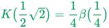
![{\displaystyle {\frac {1}{\sqrt {x^{6}+1}}}={\frac {\mathrm {d} }{\mathrm {d} x}}\,{\frac {1}{6}}{\sqrt[{4}]{27}}F{\biggl [}2\arctan {\biggl (}{\frac {{\sqrt[{4}]{3}}\,x}{\sqrt {x^{2}+1}}}{\biggr )};{\frac {1}{4}}({\sqrt {6}}+{\sqrt {2}}){\biggr ]}}](https://wikimedia.org/api/rest_v1/media/math/render/svg/3186259fdf61a7ebb632f3d02d679cae524c35f7)

![{\displaystyle {\frac {1}{6{\sqrt[{3}]{2}}}}\csc {\bigl (}{\frac {\pi }{6}}{\bigr )}\beta {\bigl (}{\frac {1}{3}}{\bigr )}=\int _{0}^{\infty }{\frac {1}{\sqrt {x^{6}+1}}}\,\mathrm {d} x={\biggl \{}{\color {blue}{\frac {1}{6}}{\sqrt[{4}]{27}}F{\biggl [}2\arctan {\biggl (}{\frac {{\sqrt[{4}]{3}}\,x}{\sqrt {x^{2}+1}}}{\biggr )};{\frac {1}{4}}({\sqrt {6}}+{\sqrt {2}}){\biggr ]}}{\biggr \}}_{x=0}^{x=\infty }=}](https://wikimedia.org/api/rest_v1/media/math/render/svg/1aeaa28cc9c443e551ccbc434cd63421302cae2b)
![{\displaystyle ={\frac {1}{6}}{\sqrt[{4}]{27}}F{\bigl [}2\arctan({\sqrt[{4}]{3}});{\frac {1}{4}}({\sqrt {6}}+{\sqrt {2}}){\bigr ]}={\frac {2}{9}}{\sqrt[{4}]{27}}K{\bigl [}{\frac {1}{4}}({\sqrt {6}}+{\sqrt {2}}){\bigr ]}={\frac {2}{3}}{\sqrt[{4}]{3}}K{\bigl [}{\frac {1}{4}}({\sqrt {6}}-{\sqrt {2}}){\bigr ]}}](https://wikimedia.org/api/rest_v1/media/math/render/svg/d55b9913617b5871c7a524c0eeec8168828a1c5a)
![{\displaystyle {\color {ForestGreen}K{\bigl [}{\frac {1}{4}}({\sqrt {6}}-{\sqrt {2}}){\bigr ]}={\frac {1}{2{\sqrt[{3}]{2}}{\sqrt[{4}]{3}}}}\beta {\bigl (}{\frac {1}{3}}{\bigr )}}}](https://wikimedia.org/api/rest_v1/media/math/render/svg/fffa258bf7309994a5d54ae0f95d4614975d1ec2)

![{\displaystyle ={\frac {\mathrm {d} }{\mathrm {d} x}}\,{\frac {1}{4}}\sec {\bigl (}{\frac {\pi }{8}}{\bigr )}F{\biggl \{}2\arctan {\biggl [}{\frac {2\cos(\pi /8)\,x}{{\sqrt {x^{4}+{\sqrt {2}}\,x^{2}+1}}-x^{2}+1}}{\biggr ]};2{\sqrt[{4}]{2}}\sin {\bigl (}{\frac {\pi }{8}}{\bigr )}{\biggr \}}+{\frac {1}{4}}\sec {\bigl (}{\frac {\pi }{8}}{\bigr )}F{\biggl \{}\arcsin {\biggl [}{\frac {2\cos(\pi /8)\,x}{x^{2}+1}}{\biggr ]};\tan {\bigl (}{\frac {\pi }{8}}{\bigr )}{\biggr \}}}](https://wikimedia.org/api/rest_v1/media/math/render/svg/9418c896b8d195e1c5bce8b760e71d95bd9cf29e)

![{\displaystyle {\frac {1}{8{\sqrt[{4}]{2}}}}\csc {\bigl (}{\frac {\pi }{8}}{\bigr )}\beta {\bigl (}{\frac {3}{8}}{\bigr )}=\int _{0}^{\infty }{\frac {1}{\sqrt {x^{8}+1}}}\,\mathrm {d} x=}](https://wikimedia.org/api/rest_v1/media/math/render/svg/21e13acda89a6825a0a7a6477bf0e2d072b3ce9e)
![{\displaystyle ={\biggl \langle }{\color {blue}{\frac {1}{4}}\sec {\bigl (}{\frac {\pi }{8}}{\bigr )}F{\biggl \{}2\arctan {\biggl [}{\frac {2\cos(\pi /8)\,x}{{\sqrt {x^{4}+{\sqrt {2}}\,x^{2}+1}}-x^{2}+1}}{\biggr ]};2{\sqrt[{4}]{2}}\sin {\bigl (}{\frac {\pi }{8}}{\bigr )}{\biggr \}}+{\frac {1}{4}}\sec {\bigl (}{\frac {\pi }{8}}{\bigr )}F{\biggl \{}\arcsin {\biggl [}{\frac {2\cos(\pi /8)\,x}{x^{2}+1}}{\biggr ]};\tan {\bigl (}{\frac {\pi }{8}}{\bigr )}{\biggr \}}}{\biggr \rangle }_{x=0}^{x=\infty }=}](https://wikimedia.org/api/rest_v1/media/math/render/svg/5ab622f4004af8bce9bb3de38a20ecb4d4219a21)
![{\displaystyle ={\frac {1}{4}}\sec {\bigl (}{\frac {\pi }{8}}{\bigr )}F{\bigl [}\pi ;2{\sqrt[{4}]{2}}\sin {\bigl (}{\frac {\pi }{8}}{\bigr )}{\bigr ]}={\frac {1}{2}}\sec {\bigl (}{\frac {\pi }{8}}{\bigr )}K({\sqrt {2{\sqrt {2}}-2}}{\bigr )}=2\sin {\bigl (}{\frac {\pi }{8}}{\bigr )}K({\sqrt {2}}-1)}](https://wikimedia.org/api/rest_v1/media/math/render/svg/85a8ad3dc4c269cf0392b1260587f5471ae5e932)
![{\displaystyle {\color {ForestGreen}K({\sqrt {2}}-1)={\frac {1}{8}}{\sqrt[{4}]{2}}\,({\sqrt {2}}+1)\,\beta {\bigl (}{\frac {3}{8}}{\bigr )}}}](https://wikimedia.org/api/rest_v1/media/math/render/svg/177a0e98ca0233f21a20d37c9dd285369ecf1cda)

![{\displaystyle q[{\tfrac {1}{4}}({\sqrt {6}}-{\sqrt {2}})]=\exp(-{\sqrt {3}}\,\pi )}](https://wikimedia.org/api/rest_v1/media/math/render/svg/93d8a66693d1cd78fa0422519e6a5f523cfa1f69)

![{\displaystyle \theta _{3}[q(k)]={\sqrt {2\pi ^{-1}K(k)}}}](https://wikimedia.org/api/rest_v1/media/math/render/svg/f5de1ea9f13775acb606c8cb4c2c8268c77ad546)
![{\displaystyle \theta _{3}[\exp(-\pi )]=\theta _{3}[q({\tfrac {1}{2}}{\sqrt {2}})]={\sqrt {2\pi ^{-1}K({\tfrac {1}{2}}{\sqrt {2}})}}=2^{-1/2}\pi ^{-1/2}\beta ({\tfrac {1}{4}})^{1/2}=2^{-1/4}{\sqrt[{4}]{\pi }}\,{\Gamma {\bigl (}{\tfrac {3}{4}}{\bigr )}}^{-1}}](https://wikimedia.org/api/rest_v1/media/math/render/svg/0c3b3090803e98069d65099cffee88f085fb58b6)
![{\displaystyle \theta _{3}[\exp(-{\sqrt {3}}\,\pi )]=\theta _{3}{\bigl \{}q{\bigl [}{\tfrac {1}{4}}({\sqrt {6}}-{\sqrt {2}}){\bigr ]}{\bigr \}}={\sqrt {2\pi ^{-1}K{\bigl [}{\tfrac {1}{4}}({\sqrt {6}}-{\sqrt {2}}){\bigr ]}}}=2^{-1/6}3^{-1/8}\pi ^{-1/2}\beta ({\tfrac {1}{3}})^{1/2}}](https://wikimedia.org/api/rest_v1/media/math/render/svg/2456d11eb2e069e9d2eac7d2cc91561418429672)
![{\displaystyle \theta _{3}[\exp(-{\sqrt {2}}\,\pi )]=\theta _{3}[q({\sqrt {2}}-1)]={\sqrt {2\pi ^{-1}K({\sqrt {2}}-1)}}=2^{-1/8}\cos({\tfrac {1}{8}}\pi )\,\pi ^{-1/2}\beta ({\tfrac {3}{8}})^{1/2}}](https://wikimedia.org/api/rest_v1/media/math/render/svg/81e6d7302b7c5a86bd706212afbf5c0dddc4be6d)
![{\displaystyle \theta _{4}[q(k)]={\sqrt[{4}]{1-k^{2}}}\,{\sqrt {2\pi ^{-1}K(k)}}}](https://wikimedia.org/api/rest_v1/media/math/render/svg/b18cb501a0e5521687946e420015ea2bfb8e9367)
![{\displaystyle \theta _{4}[\exp(-{\sqrt {2}}\,\pi )]=\theta _{4}[q({\sqrt {2}}-1)]={\sqrt[{4}]{2{\sqrt {2}}-2}}\,{\sqrt {2\pi ^{-1}K({\sqrt {2}}-1)}}=2^{-1/4}\cos({\tfrac {1}{8}}\pi )^{1/2}\,\pi ^{-1/2}\beta ({\tfrac {3}{8}})^{1/2}}](https://wikimedia.org/api/rest_v1/media/math/render/svg/07c0cdf2fb31e0ad42c1c55d8562d70da28f2203)


![{\displaystyle \sum _{k=0}^{\infty }P(k)x^{k}={\frac {1}{(x;x)_{\infty }}}=\theta _{3}(x)^{-1/6}\theta _{4}(x)^{-2/3}{\biggl [}{\frac {\theta _{3}(x)^{4}-\theta _{4}(x)^{4}}{16\,x}}{\biggr ]}^{-1/24}}](https://wikimedia.org/api/rest_v1/media/math/render/svg/d45936d0522b1f639420fa97f49e237424fa4a51)
![{\displaystyle (x;x)_{\infty }=1+\sum _{n=1}^{\infty }{\bigl [}-x^{{\text{Fn}}(2n-1)}-x^{{\text{Kr}}(2n-1)}+x^{{\text{Fn}}(2n)}+x^{{\text{Kr}}(2n)}{\bigr ]}}](https://wikimedia.org/api/rest_v1/media/math/render/svg/eab59cb2fcf2f3ddc6f1e10561a526de51f516f3)




![{\displaystyle \sum _{k=0}^{\infty }Q(k)x^{k}={\frac {1}{(x;x^{2})_{\infty }}}=\theta _{3}(x)^{1/6}\theta _{4}(x)^{-1/3}{\biggl [}{\frac {\theta _{3}(x)^{4}-\theta _{4}(x)^{4}}{16\,x}}{\biggr ]}^{1/24}}](https://wikimedia.org/api/rest_v1/media/math/render/svg/faf3d08f52a11ebbc9e5b9289d4f784f60f103d7)
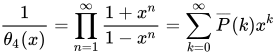



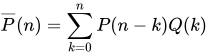
![{\displaystyle \theta _{4}(x)={\biggl [}\sum _{k=0}^{\infty }P(k)x^{k}{\biggr ]}^{-1}{\biggl [}\sum _{k=0}^{\infty }Q(k)x^{k}{\biggr ]}^{-1}}](https://wikimedia.org/api/rest_v1/media/math/render/svg/4ed01dd893d339d67b7cffd351479d11bd83f819)