In continuum mechanics, the material derivative^[1][2] describes the time rate of change of some physical quantity (like heat or momentum) of a material element that is subjected to a space-and-time-dependent macroscopic velocity field. The material derivative can serve as a link between Eulerian and Lagrangian descriptions of continuum deformation.^[3]

For example, in fluid dynamics, the velocity field is the flow velocity, and the quantity of interest might be the temperature of the fluid. In this case, the material derivative then describes the temperature change of a certain fluid parcel with time, as it flows along its pathline (trajectory).

Other names

There are many other names for the material derivative, including:

• advective derivative^[4]
• convective derivative^[5]
• derivative following the motion^[1]
• hydrodynamic derivative^[1]
• Lagrangian derivative^[6]
• particle derivative^[7]
• substantial derivative^[1]
• substantive derivative^[8]
• Stokes derivative^[8]
• total derivative,^[1][9] although the material derivative is actually a special case of the total derivative^[9]

History

The material derivative emerged during the mid-18th century, when Jean le Rond d'Alembert and Leonhard Euler first formulated hydrodynamics as a field theory governed by partial differential equations.^[10][11] Euler is believed to have been the first to write the fluid acceleration term as it is understood today, expressing the total acceleration of a fluid particle as the sum of local and convective contributions.^[12] The distinction between the two fundamental descriptions of fluid motion, i.e. the Eulerian (field) description and the Lagrangian (material) description, was established during this period. Euler introduced material coordinates in 1762, though they are now commonly called Lagrangian coordinates, while d'Alembert introduced spatial coordinates in 1752, now often called Eulerian coordinates.^[13]

The mathematical expression for the material derivative is attributed independently to Euler (around 1770) and Joseph-Louis Lagrange (around 1783).^[14] Lagrange, in his 1788 treatise *Mécanique Analytique*, further developed the Lagrangian framework for describing fluid motion, which naturally led to the concept of differentiation following a material particle.^[15]

The operator was brought to prominence in the English-speaking world by Sir George Gabriel Stokes, who introduced the now-standard ${\displaystyle D/Dt}$ notation for the material derivative in his 1845 paper on the motion of incompressible fluids.^[16][17] For this reason, the material derivative is still sometimes called the Stokes derivative.^[8]

The notation ${\displaystyle D/Dt}$ has been a subject of debate among fluid dynamicists. Stokes first used it in 1845, but it was criticized by Harold Jeffreys and Bertha Jeffreys (1946) as a relic of an obsolete 19th-century notational convention for partial derivatives.^[18][19] Some authors prefer to write the full expression ${\displaystyle \partial /\partial t+\mathbf {u} \cdot \nabla }$ without using an abbreviation, while others use ${\displaystyle d/dt}$ for Lagrangian coordinates and reserve ${\displaystyle D/Dt}$ for Eulerian coordinates.^[20][21] Defenders of the ${\displaystyle D/Dt}$ notation, including Frank M. White and James Lighthill, have argued for its continued use on the grounds of clarity and tradition.^[22][23]

The modern understanding of the material derivative as the link between Eulerian and Lagrangian descriptions was consolidated in the 20th century through the works of continuum mechanicians such as Clifford Truesdell and others.^[10][24] Today, the material derivative is a foundational concept in fluid dynamics, continuum mechanics, and related fields, appearing in the Navier–Stokes equations, the energy equation, and the conservation laws of physics.

Definition

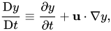
The material derivative is defined for any tensor field ${\displaystyle y}$ that is macroscopic, with the sense that it depends only on position and time coordinates, ${\displaystyle y=y(x,t)}$: $${\displaystyle {\frac {\mathrm {D} y}{\mathrm {D} t}}\equiv {\frac {\partial y}{\partial t}}+\mathbf {u} \cdot \nabla y,}$$ where ${\displaystyle \nabla y}$ is the covariant derivative of the tensor, and ${\displaystyle \mathbf {u} (x,t)}$ is the flow velocity. Generally the convective derivative of the field ${\displaystyle \mathbf {u} \cdot \nabla y}$, the one that contains the covariant derivative of the field, can be interpreted both as involving the streamline tensor derivative of the field ${\displaystyle \mathbf {u} \cdot \nabla y}$, or as involving the streamline directional derivative of the field ${\displaystyle (\mathbf {u} \cdot \nabla )\ y}$, leading to the same result.^[25] Only this spatial term containing the flow velocity describes the transport of the field in the flow, while the other describes the intrinsic variation of the field, independent of the presence of any flow. Confusingly, sometimes the name "convective derivative" is used for the whole material derivative ${\displaystyle \mathrm {D} /\mathrm {D} t}$, instead for only the spatial term ${\displaystyle \mathbf {u} \cdot \nabla }$.^[2] The effect of the time-independent terms in the definitions are for the scalar and tensor case respectively known as advection and convection.

Development via the total derivative

Consider a scalar quantity ${\displaystyle \phi (\mathbf {x} ,t)}$, where ${\displaystyle t}$ is time and ${\displaystyle \mathbf {x} }$ is position. Here ${\displaystyle \phi }$ may be some physical variable such as temperature or chemical concentration. The physical quantity, whose scalar quantity is ${\displaystyle \phi }$, exists in a continuum, and whose macroscopic velocity is represented by the vector field ${\displaystyle \mathbf {u} (\mathbf {x} ,t)}$.

The (total) derivative with respect to time of ${\displaystyle \phi }$ is expanded using the multivariate chain rule: $${\displaystyle {\frac {\mathrm {d} }{\mathrm {d} t}}\phi (\mathbf {x} (t),t)={\frac {\partial \phi }{\partial t}}+{\dot {\mathbf {x} }}\cdot \nabla \phi .}$$

It is apparent that this derivative is dependent on the vector $${\displaystyle {\dot {\mathbf {x} }}\equiv {\frac {\mathrm {d} \mathbf {x} }{\mathrm {d} t}},}$$ which describes a chosen path ${\displaystyle \mathbf {x} (t)}$ in space. For example, if ${\displaystyle {\dot {\mathbf {x} }}=\mathbf {0} }$ is chosen, the time derivative becomes equal to the partial time derivative, which agrees with the definition of a partial derivative: a derivative taken with respect to some variable (time in this case) holding other variables constant (space in this case). This makes sense because if ${\displaystyle {\dot {\mathbf {x} }}=0}$, then the derivative is taken at some constant position. This static position derivative is called the Eulerian derivative.

An example of this case is a swimmer standing still and sensing temperature change in a lake early in the morning: the water gradually becomes warmer due to heating from the sun. In which case the term ${\displaystyle {\partial \phi }/{\partial t}}$ is sufficient to describe the rate of change of temperature.

If the sun is not warming the water (i.e. ${\displaystyle {\partial \phi }/{\partial t}=0}$), but the path ${\displaystyle \mathbf {x} (t)}$ is not a standstill, the time derivative of ${\displaystyle \phi }$ may change due to the path. For example, imagine the swimmer is in a motionless pool of water, indoors and unaffected by the sun. One end happens to be at a constant high temperature and the other end at a constant low temperature. By swimming from one end to the other the swimmer senses a change of temperature with respect to time, even though the temperature at any given (static) point is a constant. This is because the derivative is taken at the swimmer's changing location and the second term on the right ${\displaystyle {\dot {\mathbf {x} }}\cdot \nabla \phi }$ is sufficient to describe the rate of change of temperature. A temperature sensor attached to the swimmer would show temperature varying with time, simply due to the temperature variation from one end of the pool to the other.

The material derivative finally is obtained when the path ${\displaystyle \mathbf {x} (t)}$ is chosen to have a velocity equal to the fluid velocity $${\displaystyle {\dot {\mathbf {x} }}=\mathbf {u} .}$$

That is, the path follows the fluid current described by the fluid's velocity field ${\displaystyle \mathbf {u} }$. So, the material derivative of the scalar ${\displaystyle \phi }$ is $${\displaystyle {\frac {\mathrm {D} \phi }{\mathrm {D} t}}={\frac {\partial \phi }{\partial t}}+\mathbf {u} \cdot \nabla \phi .}$$

Geometrical interpretation

An intuitive, geometrical understanding of the material derivative was provided by Moots and Mavis (1938) in their study of flood waves.^[26] They considered a scalar quantity (such as flow velocity ${\displaystyle u}$) as a function of space ${\displaystyle x}$ and time ${\displaystyle t}$, represented by a surface ${\displaystyle u=f(x,t)}$ in three-dimensional space (Figure 3).

[[File:Material_Derivative_3 thumb .jpg|thumb|right|400px|Figure 3: Geometrical interpretation of the material derivative. The surface ${\displaystyle u=f(x,t)}$ shows the velocity field. The curve ${\displaystyle LMN}$ traces the path of a fluid particle (${\displaystyle dx/dt=u}$), and the total derivative ${\displaystyle du/dt}$ is the slope of the tangent to the projected curve ${\displaystyle GHI}$.^[26]]]

In this geometric view:

• The curve ${\displaystyle APB}$ is the intersection of the surface ${\displaystyle u=f(x,t)}$ with a plane of constant ${\displaystyle x}$. The slope of the tangent to this curve at any point gives the partial derivative ${\displaystyle \partial u/\partial t}$, which is the local rate of change at a fixed spatial location.
• The curve ${\displaystyle CPD}$ is the intersection of the surface with a plane of constant ${\displaystyle t}$ (a "snapshot" of the field). The slope of the tangent to this curve gives the spatial gradient ${\displaystyle \partial u/\partial x}$.
• The curve ${\displaystyle EPF}$ lies on the surface and represents the path of a fluid particle moving with velocity ${\displaystyle u=dx/dt}$. The total derivative ${\displaystyle du/dt}$ is the slope of the tangent to this space curve projected onto the ${\displaystyle ut}$-plane (the curve ${\displaystyle GHI}$).

This visualization clearly demonstrates that the material derivative ${\displaystyle du/dt}$ is not merely an abstract sum, but the actual rate of change experienced by a physical particle. The difference between the slopes of ${\displaystyle GHI}$ (total) and ${\displaystyle KHJ}$ (local, ${\displaystyle \partial u/\partial t}$) is precisely the convective contribution ${\displaystyle u\,\partial u/\partial x}$.^[26]

Application to unsteady open-channel flow

The practical power of the material derivative is illustrated by its application to flood waves in wide rectangular channels, as developed by Moots and Mavis (1938).^[26] In this context, the flow is unsteady, meaning that quantities such as velocity ${\displaystyle u}$, depth ${\displaystyle h}$, and discharge per unit width ${\displaystyle q=hu}$ depend on both position ${\displaystyle x}$ and time ${\displaystyle t}$.

The equation of motion for a fluid element (Figure 2) was derived by equating the net pressure force, gravity component, and friction force to the mass times acceleration:^[26] $${\displaystyle \rho h\,dx{\frac {du}{dt}}=-wh{\frac {\partial h}{\partial x}}dx+wh\left(S-{\frac {Ku^{2}}{h}}\right)dx,}$$ which simplifies to: $${\displaystyle {\frac {du}{dt}}=-g{\frac {\partial h}{\partial x}}+g\left(S-{\frac {Ku^{2}}{h}}\right).}$$ Here, the acceleration of the fluid particle is written using the material derivative: $${\displaystyle {\frac {du}{dt}}={\frac {\partial u}{\partial t}}+u{\frac {\partial u}{\partial x}}.}$$ The term ${\displaystyle \partial u/\partial t}$ represents the local acceleration at a fixed station, while ${\displaystyle u\,\partial u/\partial x}$ is the convective acceleration as the particle moves to a region of different velocity.

Coupled with this is the equation of continuity (Figure 1), which states that the difference between inflow and outflow over a small reach equals the change in storage:^[26] $${\displaystyle {\frac {\partial q}{\partial x}}+{\frac {\partial h}{\partial t}}=0,\quad {\text{or}}\quad h{\frac {\partial u}{\partial x}}+u{\frac {\partial h}{\partial x}}+{\frac {\partial h}{\partial t}}=0.}$$

Using these equations, the authors derived several important results for flood waves:^[26]

• The **virtual velocity** of a constant discharge ${\displaystyle q}$ is given by ${\displaystyle V_{q}=u+h\,(\partial u/\partial t)/(\partial h/\partial t)}$, showing that the wave speed can exceed, equal, or even be less than the fluid velocity, and may become infinite or change sign at certain stages of the flood.
• The **profile of a monoclinal (rising) flood wave** was obtained in closed form by integrating the equations, demonstrating how the wave front gradually steepens or flattens.
• For a **small-amplitude wave**, the wave speed approaches ${\displaystyle V={\frac {3}{2}}u}$, which is greater than the mean flow velocity.
• For a **roll wave** (a wave moving without change of form), the wave speed equals the mean fluid velocity, ${\displaystyle V=u}$.

These classical results highlight the necessity of using the material derivative (rather than just the local derivative) to correctly capture the dynamics of rapidly varying flows, such as those encountered during floods.

Orthogonal coordinates

It may be shown that, in orthogonal coordinates, the ${\displaystyle j}$-th component of the convection term of the material derivative of a vector field ${\displaystyle \mathbf {A} }$ is given by^[27] $${\displaystyle [\left(\mathbf {u} \cdot \nabla \right)\mathbf {A} ]_{j}=\sum _{i}{\frac {u_{i}}{h_{i}}}{\frac {\partial A_{j}}{\partial q^{i}}}+{\frac {A_{i}}{h_{i}h_{j}}}\left(u_{j}{\frac {\partial h_{j}}{\partial q^{i}}}-u_{i}{\frac {\partial h_{i}}{\partial q^{j}}}\right),}$$

where the ${\displaystyle h_{i}}$ are related to the metric tensors by ${\displaystyle h_{i}={\sqrt {g_{ii}}}.}$

In the special case of a three-dimensional Cartesian coordinate system ${\displaystyle (x,y,z)}$, and ${\displaystyle \mathbf {A} }$ being a 1-tensor (a vector with three components), this is just: $${\displaystyle (\mathbf {u} \cdot \nabla )\mathbf {A} ={\begin{pmatrix}\displaystyle u_{x}{\frac {\partial A_{x}}{\partial x}}+u_{y}{\frac {\partial A_{x}}{\partial y}}+u_{z}{\frac {\partial A_{x}}{\partial z}}\\\displaystyle u_{x}{\frac {\partial A_{y}}{\partial x}}+u_{y}{\frac {\partial A_{y}}{\partial y}}+u_{z}{\frac {\partial A_{y}}{\partial z}}\\\displaystyle u_{x}{\frac {\partial A_{z}}{\partial x}}+u_{y}{\frac {\partial A_{z}}{\partial y}}+u_{z}{\frac {\partial A_{z}}{\partial z}}\end{pmatrix}}={\frac {\partial (A_{x},A_{y},A_{z})}{\partial (x,y,z)}}\mathbf {u} }$$

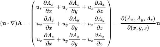
where ${\displaystyle {\frac {\partial (A_{x},A_{y},A_{z})}{\partial (x,y,z)}}}$ is a Jacobian matrix.

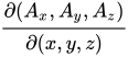
There is also a vector-dot-del identity for the case ${\displaystyle \mathbf {u} =\mathbf {A} }$, for which the material derivative for a vector field ${\displaystyle \mathbf {A} }$ can be expressed as:

${\displaystyle {\displaystyle (\mathbf {A} \cdot \nabla )\mathbf {A} ={\frac {1}{2}}\nabla |\mathbf {A} |^{2}-\mathbf {A} \times (\nabla \times \mathbf {A} )={\frac {1}{2}}\nabla |\mathbf {A} |^{2}+(\nabla \times \mathbf {A} )\times \mathbf {A} }.}$

See also

References

Further reading

• Cohen, Ira M.; Kundu, Pijush K (2008). Fluid Mechanics (4th ed.). Academic Press. ISBN 978-0-12-373735-9.
• Lai, Michael; Krempl, Erhard; Ruben, David (2010). Introduction to Continuum Mechanics (4th ed.). Elsevier. ISBN 978-0-7506-8560-3.

References

- 1 2 3 4 5 Bird, R.B.; Stewart, W.E.; Lightfoot, E.N. (2007). Transport Phenomena (Revised Second ed.). John Wiley & Sons. p. 83. ISBN 978-0-470-11539-8.
- 1 2 Batchelor, G. K. (1967). An Introduction to Fluid Dynamics. Cambridge University Press. pp. 72–73. ISBN 0-521-66396-2.
- ↑ Trenberth, K. E. (1993). Climate System Modeling. Cambridge University Press. p. 99. ISBN 0-521-43231-6.
- ↑ Majda, A. (2003). Introduction to PDEs and Waves for the Atmosphere and Ocean. Courant Lecture Notes in Mathematics. Vol. 9. American Mathematical Society. p. 1. ISBN 0-8218-2954-8.
- ↑ Ockendon, H.; Ockendon, J.R. (2004). Waves and Compressible Flow. Springer. p. 6. ISBN 0-387-40399-X.
- ↑ Mellor, G.L. (1996). Introduction to Physical Oceanography. Springer. p. 19. ISBN 1-56396-210-1.
- ↑ Stoker, J.J. (1992). Water Waves: The Mathematical Theory with Applications. Wiley. p. 5. ISBN 0-471-57034-6.
- 1 2 3 Granger, R.A. (1995). Fluid Mechanics. Courier Dover Publications. p. 30. ISBN 0-486-68356-7.
- 1 2 Landau, L.D.; Lifshitz, E.M. (1987). Fluid Mechanics. Course of Theoretical Physics. Vol. 6 (2nd ed.). Butterworth-Heinemann. pp. 3–4 & 227. ISBN 0-7506-2767-0.
- 1 2 Truesdell, C. (1954). The Kinematics of Vorticity. Indiana University Press.
- ↑ Darrigol, Olivier (2005). Worlds of Flow: A History of Hydrodynamics from the Bernoullis to Prandtl. Oxford University Press. ISBN 978-0-19-856843-8.
- ↑ "Invitation to Hydrodynamics". Retrieved 2026-08-26.
- ↑ Truesdell, C. (1952). "The Mechanical Foundations of Elasticity and Fluid Dynamics". Journal of Rational Mechanics and Analysis. 1: 125–300.
- ↑ Encyclopedia of Fluid Mechanics. Gulf Publishing Company. 1986.
- ↑ Lagrange, Joseph-Louis (1788). Mécanique Analytique.
- ↑ Stokes, G. G. (1845). "On the Theories of the Internal Friction of Fluids in Motion, and of the Equilibrium and Motion of Elastic Solids". Transactions of the Cambridge Philosophical Society. 8: 287–319.
- ↑ Stokes, G. G. (1851). "On the Effect of the Internal Friction of Fluids on the Motion of Pendulums". Transactions of the Cambridge Philosophical Society. 9: 8–106.
- ↑ Jeffreys, Harold; Jeffreys, Bertha (1946). Methods of Mathematical Physics. Cambridge University Press.
- ↑ Cajori, Florian (1929). A History of Mathematical Notations. Open Court.
- ↑ Saffman, Philip G. (1992). Vortex Dynamics. Cambridge University Press. ISBN 978-0-521-47739-0.
- ↑ Tong, Christopher H. (2024). D/Dt or d/dt for the material derivative? The views of Sir George, Sir Harold, Lady Bertha, Sir James, and other friends. 77th Annual Meeting of the APS Division of Fluid Dynamics.
- ↑ White, Frank M. (2006). Viscous Fluid Flow (3rd ed.). McGraw-Hill. ISBN 978-0-07-124493-0.
- ↑ Lighthill, James (1986). An Informal Introduction to Theoretical Fluid Mechanics. Clarendon Press. ISBN 978-0-19-853630-7.
- ↑ Truesdell, C.; Toupin, R. (1960). "The Classical Field Theories". Handbuch der Physik. Vol. III/1. Springer.
- ↑ Emanuel, G. (2001). Analytical fluid dynamics (second ed.). CRC Press. pp. 6–7. ISBN 0-8493-9114-8.
- 1 2 3 4 5 6 7 8 Moots, E. E.; Mavis, F. T. (1938). A study in flood waves. State University of Iowa. pp. 6–9. doi:10.17077/0062-02.
- ↑ Eric W. Weisstein. "Convective Operator". MathWorld. Retrieved 2008-07-22.